Detect Autocorrelation
Visually detect autocorrelation in a time series by plotting stem plots of the sample
autocorrelation and partial autocorrelation functions (ACF and PACF, respectively), using
autocorr and parcorr. Conduct a statistical test that detects
autocorrelation effects in a time series by conducting a Ljung-Box Q-test using lbqtest.
Compute Sample ACF and PACF
Visually and qualitatively assess autocorrelation in a time series is 57 consecutive days of overshorts from a gasoline tank in Colorado by computing and plotting the sample ACF and PACF.
Load Data
Load the time series of overshorts.
load Data_Overshort
y = Data;
n = length(y);

figure
plot(y)
xlim([0 n])
title("Overshorts for 57 Consecutive Days")

The series appears to be stationary.
Plot Sample ACF and PACF
Plot the sample ACF and PACF.
figure
tiledlayout(2,1)
nexttile
autocorr(y)
nexttile
parcorr(y)
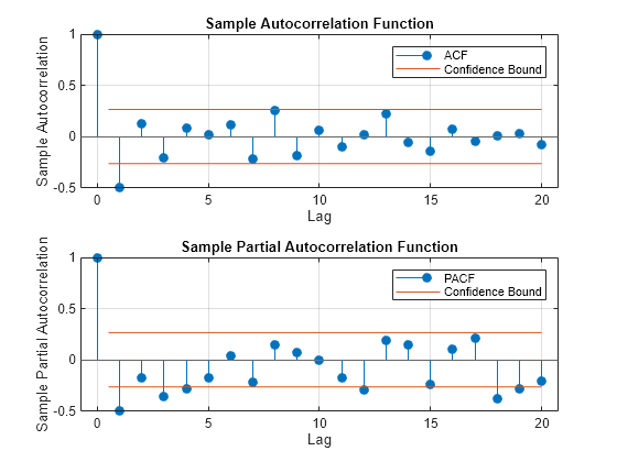
The sample ACF and PACF exhibit significant autocorrelation. The sample ACF has significant autocorrelation at lag 1. The sample PACF has significant autocorrelation at lags 1, 3, and 4.
The distinct cutoff of the ACF combined with the more gradual decay of the PACF suggests an MA(1) model might be appropriate for this data.
Store Sample ACF and PACF Values
Set variables to the sample ACF and PACF values up to lag 15.
acf = autocorr(y,NumLags=15);
pacf = parcorr(y,NumLags=15);
[length(acf) length(pacf)]
ans = 1×2

    16    16
The outputs acf and pacf are vectors storing the sample autocorrelation and partial autocorrelation at lags 0, 1,...,15 (a total of 16 lags).
Conduct the Ljung-Box Q-Test
Assess autocorrelation in a time series is 57 consecutive days of overshorts from a gasoline tank in Colorado by conducting the Ljung-Box Q-test for autocorrelation.
Load Data
Load the time series of overshorts.
load Data_Overshort
y = Data;
n = length(y);

figure
plot(y)
xlim([0 n])
title("Overshorts for 57 Consecutive Days")

The data appears to fluctuate around a constant mean, so no data transformations are needed before conducting the Ljung-Box Q-test.
Conduct the Ljung-Box Q-test.
Conduct the Ljung-Box Q-test for autocorrelation at lags 5, 10, and 15.
[h,p,Qstat,crit] = lbqtest(y,Lags=[5 10 15])
h = 1×3 logical array

   1   1   1
p = 1×3

    0.0016    0.0007    0.0013
Qstat = 1×3

   19.3604   30.5986   36.9639
crit = 1×3

   11.0705   18.3070   24.9958
All outputs are vectors with three elements, corresponding to tests at each of the three lags. The first element of each output corresponds to the test at lag 5, the second element corresponds to the test at lag 10, and the third element corresponds to the test at lag 15.
The test decisions are stored in the vector h. The value h = 1 means reject the null hypothesis. Vector p contains the p-values for the three tests. At the significance level, the null hypothesis of no autocorrelation is rejected at all three lags. The conclusion is that there is significant autocorrelation in the series.
The test statistics and critical values are given in outputs Qstat and crit, respectively.
What Is the Ljung-Box Q-Test?
The sample autocorrelation function (ACF) and partial autocorrelation function (PACF) are useful qualitative tools to assess the presence of autocorrelation at individual lags. The Ljung-Box Q-test is a more quantitative way to test for autocorrelation at multiple lags jointly [3]. The null hypothesis for this test is that the first m autocorrelations are jointly zero,
The choice of m affects test performance. If N is the length of your observed time series, choosing is recommended for power [4]. You can test at multiple values of m. If seasonal autocorrelation is possible, you might consider testing at larger values of m, such as 10 or 15.
The Ljung-Box test statistic is given by
This is a modification of the Box-Pierce Portmanteau “Q” statistic [1]. Under the null hypothesis, Q(m) follows a distribution.
You can use the Ljung-Box Q-test to assess autocorrelation in any series with a constant
mean. This includes residual series, which can be tested for autocorrelation during model
diagnostic checks. If the residuals result from fitting a model with g
parameters, you should compare the test statistic to a distribution with m – g degrees of
freedom. Optional input arguments to lbqtest let you modify the degrees
of freedom of the null distribution.
You can also test for conditional heteroscedasticity by conducting a Ljung-Box Q-test on
a squared residual series. An alternative test for conditional heteroscedasticity is Engle’s
ARCH test (archtest).
References
[1] Box, G. E. P. and D. Pierce. “Distribution of Residual Autocorrelations in Autoregressive-Integrated Moving Average Time Series Models.” Journal of the American Statistical Association. Vol. 65, 1970, pp. 1509–1526.
[2] Brockwell, P. J. and R. A. Davis. Introduction to Time Series and Forecasting. 2nd ed. New York, NY: Springer, 2002.
[3] Ljung, G. and G. E. P. Box. “On a Measure of Lack of Fit in Time Series Models.” Biometrika. Vol. 66, 1978, pp. 67–72.
[4] Tsay, R. S. Analysis of Financial Time Series. 3rd ed. Hoboken, NJ: John Wiley & Sons, Inc., 2010.
See Also
Apps
Functions
Topics
- Detect Serial Correlation Using Econometric Modeler App
- Detect ARCH Effects Using Econometric Modeler App
- Detect ARCH Effects
- Choose ARMA Lags Using BIC
- Create Seasonal ARIMA (SARIMA) Model for Time Series Data
- Specify Conditional Mean and Variance Models
- Autocorrelation and Partial Autocorrelation
- What Are Moving Average (MA) Models?
- Goodness of Fit