diffusion
Diffusion-rate model component
Description
The diffusion object specifies the diffusion-rate component
of continuous-time stochastic differential equations (SDEs).
The diffusion-rate specification supports the simulation of sample paths of
NVars state variables driven by NBrowns
Brownian motion sources of risk over NPeriods consecutive observation
periods, approximating continuous-time stochastic processes.
The diffusion-rate specification can be any
NVars-by-NBrowns matrix-valued function
G of the general form:
| (1) |
Dis anNVars-by-NVarsdiagonal matrix-valued function.Each diagonal element of
Dis the corresponding element of the state vector raised to the corresponding element of an exponentAlpha, which is anNVars-by-1vector-valued function.Vis anNVars-by-NBrownsmatrix-valued volatility rate functionSigma.AlphaandSigmaare also accessible using the (t, Xt) interface.
And a diffusion-rate specification is associated with a vector-valued SDE of the form:
where:
Xt is an
NVars-by-1state vector of process variables.dWt is an
NBrowns-by-1Brownian motion vector.D is an
NVars-by-NVarsdiagonal matrix, in which each element along the main diagonal is the corresponding element of the state vector raised to the corresponding power of α.V is an
NVars-by-NBrownsmatrix-valued volatility rate functionSigma.
The diffusion-rate specification is flexible, and provides direct parametric support for static volatilities and state vector exponents. It is also extensible, and provides indirect support for dynamic/nonlinear models via an interface. This enables you to specify virtually any diffusion-rate specification.
Creation
Description
DiffusionRate = diffusion(Alpha,Sigma)DiffusionRate model component.
Specify required input parameters A and
B as one of the following types:
A MATLAB® array. Specifying an array indicates a static (non-time-varying) parametric specification. This array fully captures all implementation details, which are clearly associated with a parametric form.
A MATLAB function. Specifying a function provides indirect support for virtually any static, dynamic, linear, or nonlinear model. This parameter is supported via an interface, because all implementation details are hidden and fully encapsulated by the function.
Note
You can specify combinations of array and function input parameters as needed.
Moreover, a parameter is identified as a deterministic function
of time if the function accepts a scalar time t
as its only input argument. Otherwise, a parameter is assumed to be
a function of time t and state
X(t) and is invoked with both input
arguments.
The diffusion object that you create encapsulates the
composite drift-rate specification and returns the following displayed parameters:
Rate— The diffusion-rate function, G.Rateis the diffusion-rate calculation engine. It accepts the current time t and anNVars-by-1state vector Xt as inputs, and returns anNVars-by-1diffusion-rate vector.Alpha— Access function for the input argumentAlpha.Sigma— Access function for the input argumentSigma.
Input Arguments
Output Arguments
Properties
Examples
More About
There are inheritance relationships among the SDE classes.
The following figure illustrates the inheritance relationships.
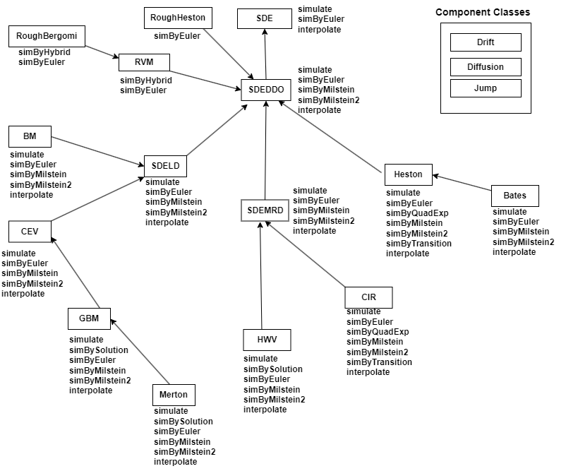
For more information, see SDE Class Hierarchy.
Algorithms
When you specify the input arguments Alpha and
Sigma as MATLAB arrays, they are associated with a specific parametric form. By contrast,
when you specify either Alpha or Sigma as a
function, you can customize virtually any diffusion-rate specification.
Accessing the output diffusion-rate parameters Alpha and
Sigma with no inputs simply returns the original input
specification. Thus, when you invoke diffusion-rate parameters with no inputs, they
behave like simple properties and allow you to test the data type (double vs. function,
or equivalently, static vs. dynamic) of the original input specification. This is useful
for validating and designing methods.
When you invoke diffusion-rate parameters with inputs, they behave like functions,
giving the impression of dynamic behavior. The parameters Alpha and
Sigma accept the observation time t and a
state vector Xt, and return an array of
appropriate dimension. Specifically, parameters Alpha and
Sigma evaluate the corresponding diffusion-rate component. Even
if you originally specified an input as an array, diffusion treats it
as a static function of time and state, by that means guaranteeing that all parameters
are accessible by the same interface.
References
[1] Aït-Sahalia, Yacine. “Testing Continuous-Time Models of the Spot Interest Rate.” Review of Financial Studies, vol. 9, no. 2, Apr. 1996, pp. 385–426.
[2] Aït-Sahalia, Yacine. “Transition Densities for Interest Rate and Other Nonlinear Diffusions.” The Journal of Finance, vol. 54, no. 4, Aug. 1999, pp. 1361–95.
[3] Glasserman, Paul. Monte Carlo Methods in Financial Engineering. Springer, 2004.
[4] Hull, John. Options, Futures and Other Derivatives. 7th ed, Prentice Hall, 2009.
[5] Johnson, Norman Lloyd, et al. Continuous Univariate Distributions. 2nd ed, Wiley, 1994.
[6] Shreve, Steven E. Stochastic Calculus for Finance. Springer, 2004.
Version History
Introduced in R2008a