Main Content

ddensd

Solve delay differential equations (DDEs) of neutral type

Description

example

sol = ddensd(ddefun,dely,delyp,history,tspan) integrates a system of delay differential equations of neutral type, that has the form

y '(t) = f(t, y(t), y(dy1),..., y(dyp), y '(dyp1),..., y '(dypq))(1)
where

  • t is the independent variable representing time.

  • dyi is any of p solution delays.

  • dypj is any of q derivative delays.

sol = ddensd(ddefun,dely,delyp,history,tspan,options) replaces default integration parameters with those specified in options, a structure created with the ddeset function.

Examples

collapse all

Solve the following neutral DDE, presented by Paul, for $0 \le t \le \pi$.

$$y'(t) = 1 + y(t) - 2y(t/2)^2 - y'(t-\pi)$$

The solution history is $y(t) = \cos(t)$ for $t \le 0$.

Create a new program file in the editor. This file will contain a main function and four local functions.

Define the first-order DDE as a local function named ddefun.

function yp = ddefun(t,y,ydel,ypdel) 
    yp = 1 + y - 2*ydel^2 - ypdel;
end

Define the solution delay as a local function named dely.

function dy = dely(t,y) 
    dy = t/2;
end

Define the derivative delay as a local function named delyp.

function dyp = delyp(t,y) 
    dyp = t-pi;
end

Define the solution history as a local function named history.

function y = history(t)
    y = cos(t);
end

Define the interval of integration and solve the DDE using ddensd. Add this code to the main function.

tspan = [0 pi];
sol = ddensd(@ddefun,@dely,@delyp,@history,tspan);

Evaluate the solution at 100 equally spaced points between $0$ and $\pi$. Add this code to the main function.

tn = linspace(0,pi);
yn = deval(sol,tn);

Plot the results. Add this code to the main function.

plot(tn,yn);
xlim([0 pi]);
ylim([-1.2 1.2]);
xlabel('time t');
ylabel('solution y');

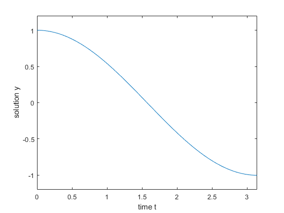
Run your entire program to calculate the solution and display the plot. The file ddex4.m contains the complete code for this example. To see the code in an editor, type edit ddex4 at the command line.

Input Arguments

collapse all

Derivative function, specified as a function handle whose syntax is yp = ddefun(t,y,ydel,ypdel). The arguments for ddefun are described in the table below.

ddefun ArgumentDescription
tA scalar value representing the current value of time, t.
y A vector that represents y(t) in Equation 1. The size of this vector is n-by-1, where n is the number of equations in the system you want to solve.
ydelA matrix whose columns, ydel(:,i), represent y(dyi). The size of this matrix is n-by-p, where n is the number of equations in the system you want to solve, and p is the number of y(dy) terms in Equation 1.
ypdelA matrix whose columns, ypdel(:,j) represent y '(dypj). The size of this matrix is n-by-q, where n is the number of equations in the system you want to solve, and q is the number of y '(dyp) terms in Equation 1.
ypThe result returned by ddefun. It is an n-by-1 vector whose elements represent the right side of Equation 1.

Solution delays, specified as a function handle, which returns dy1,..., dyp in Equation 1. Alternatively, you can pass constant delays in the form of a vector.

If you specify dely as a function handle, the syntax must be dy = dely(t,y). The arguments for this function are described in the table below.

dely ArgumentDescription
tA scalar value representing the current value of time, t.
yA vector that represents y(t) in Equation 1. The size of this vector is n-by-1, where n is the number of equations in the system you want to solve.
dyA vector returned by the dely function whose values are the solution delays, dyi , in Equation 1. The size of this vector is p-by-1, where p is the number of solution delays in the equation. Each element must be less than or equal to t.

If you want to specify constant solution delays having the form dyi = tτi, then dely must be a vector, where dely(i) = τi. Each value in this vector must be greater than or equal to zero.

If dy is not present in the problem, set dely to [].

Data Types: function_handle | single | double

Derivative delays, specified as a function handle, which returns dyp1,..., dypq in Equation 1. Alternatively, you can pass constant delays in the form of a vector.

If delyp is a function handle, its syntax must be dyp = delyp(t,y). The arguments for this function are described in the table below.

delyp ArgumentDescription
tA scalar value representing the current value of time, t.
yA vector that represents y(t) in Equation 1. The size of this vector is n-by-1, where n is the number of equations in the system you want to solve.
dypA vector returned by the delyp function whose values are the derivative delays, dypj, in Equation 1. The size of this vector must be q-by-1, where q is the number of solution delays, dypj, in the equation. Each element of dyp must be less than t. There is one exception to this restriction: if you are solving an initial value DDE, the value of dyp can equal t at t = t0. For more information, see Initial Value Neutral Delay Differential Equations.

If you want specify constant derivative delays having the form dypj = tτj, then delyp must be a vector, where delyp(j) = τj. Each value in this vector must be greater than zero. An exception to this restriction occurs when you solve initial value problems for DDEs of neutral type. In such cases, a value in delyp can equal zero at t = t0. See Initial Value Neutral Delay Differential Equations for more information.

If dyp is not present in the problem, set delyp to [].

Data Types: function_handle | single | double

Solution history, specified as a function handle, column vector, sol structure (from a previous integration), or a cell array. This is the solution at tt0.

  • If the history varies with time, specify the solution history as a function handle whose syntax is y = history(t). This function returns an n-by-1 vector that approximates the solution, y(t), for t <= t0. The length of this vector, n, is the number of equations in the system you want to solve.

  • If y(t) is constant, you can specify history as an n-by-1 vector of the constant values.

  • If you are calling ddensd to continue a previous integration to t0, you can specify history as the output, sol, from the previous integration.

  • If you are solving an initial value DDE, specify history as a cell array, {y0, yp0}. The first element, y0, is a column vector of initial values, y(t0). The second element, yp0, is a column vector whose elements are the initial derivatives, y '(t0). These vectors must be consistent, meaning that they satisfy Equation 1 at t0. See Initial Value Neutral Delay Differential Equations for more information.

Data Types: function_handle | single | double | struct | cell

Interval of integration, specified as the vector [t0 tf]. The first element, t0, is the initial value of t. The second element, tf, is the final value of t. The value of t0 must be less than tf.

Data Types: single | double

Optional integration parameters, specified as a structure created and returned by the ddeset function. Some commonly used properties are: 'RelTol', 'AbsTol', and 'Events'. See the ddeset reference page for more information about specifying options.

Output Arguments

collapse all

Solution, returned as a structure containing the following fields.

sol.xMesh selected by ddensd.
sol.yAn approximation to y(t) at the mesh points.
sol.ypAn approximation to y '(t) at the mesh points.
sol.solverA character vector identifying the solver, 'ddensd'.

You can pass sol to the deval function to evaluate the solution at specific points. For example, y = deval(sol, 0.5*(sol.x(1) + sol.x(end))) evaluates the solution at the midpoint of the interval of integration.

More About

collapse all

Initial Value Neutral Delay Differential Equations

An initial value DDE has dyit0 and dypjt0, for all i and j. At t = t0, all delayed terms reduce to y(dyi) = y(t0) and y '(dypj) = y '(t0):

y '(t0) = f(t0, y(t0), y(t0),..., y(t0), y '(t0),..., y '(t0))(2)
For t > t0, all derivative delays must satisfy dyp < t.

When you solve initial value neutral DDEs, you must supply y '(t0) to ddensd. To do this, specify history as a cell array {Y0,YP0}. Here, Y0 is the column vector of initial values, y(t0), and YP0 is a column vector of initial derivatives, y '(t0). These vectors must be consistent, meaning that they satisfy Equation 2 at t0.

Algorithms

For information about the algorithm used in this solver, see Shampine [2].

References

[1] Paul, C.A.H. “A Test Set of Functional Differential Equations.” Numerical Analysis Reports. No. 243. Manchester, UK: Math Department, University of Manchester, 1994.

[2] Shampine, L.F. “Dissipative Approximations to Neutral DDEs.” Applied Mathematics & Computation. Vol. 203, Number 2, 2008, pp. 641–648.

Version History

Introduced in R2012b