gradient
Numerical gradient
Syntax
Description
FX = gradient(F)F. The output FX corresponds
to ∂F/∂x, which
are the differences in the x (horizontal) direction.
The spacing between points is assumed to be 1.
[ returns the x and y components
of the two-dimensional numerical
gradient of matrix FX,FY]
= gradient(F)F. The additional output FY corresponds
to ∂F/∂y, which
are the differences in the y (vertical) direction.
The spacing between points in each direction is assumed to be 1.
Examples
Calculate the gradient of a monotonically increasing vector.
x = 1:10
x = 1×10

     1     2     3     4     5     6     7     8     9    10
fx = gradient(x)
fx = 1×10

     1     1     1     1     1     1     1     1     1     1
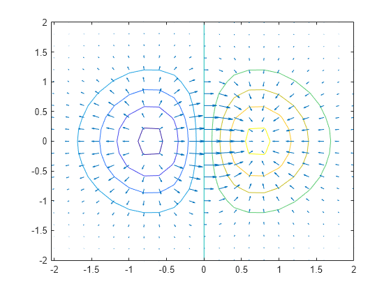
Calculate the 2-D gradient of on a grid.
x = -2:0.2:2;
y = x';
z = x .* exp(-x.^2 - y.^2);
[px,py] = gradient(z);
Plot the contour lines and vectors in the same figure.
figure
contour(x,y,z)
hold on
quiver(x,y,px,py)
hold off
Use the gradient at a particular point to linearly approximate the function value at a nearby point and compare it to the actual value.
The equation for linear approximation of a function value is
That is, if you know the value of a function and the slope of the derivative at a particular point , then you can use this information to approximate the value of the function at a nearby point .
Calculate some values of the sine function between -1 and 0.5. Then calculate the gradient.
y = sin(-1:0.25:0.5);
yp = gradient(y,0.25);
Use the function value and derivative at x = 0.5 to predict the value of sin(0.5005).
y_guess = y(end) + yp(end)*(0.5005 - 0.5)
y_guess =
0.4799
Compute the actual value for comparison.
y_actual = sin(0.5005)
y_actual =
0.4799
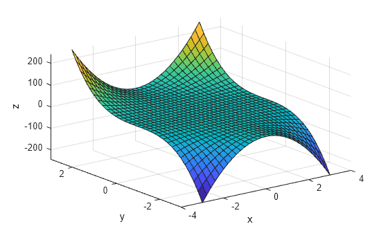
Find the value of the gradient of a multivariate function at a specified point.
Consider the multivariate function .
x = -3:0.2:3;
y = x';
f = x.^2 .* y.^3;
surf(x,y,f)
xlabel('x')
ylabel('y')
zlabel('z')
Calculate the gradient on the grid.
[fx,fy] = gradient(f,0.2);
Extract the value of the gradient at the point (1,-2). To do this, first obtain the indices of the point you want to work with. Then, use the indices to extract the corresponding gradient values from fx and fy.
x0 = 1;
y0 = -2;
t = (x == x0) & (y == y0);
indt = find(t);
f_grad = [fx(indt) fy(indt)]
f_grad = 1×2

  -16.0000   12.0400
The exact value of the gradient of at the point (1,-2) is
Input Arguments
Output Arguments
More About
Tips
Use
diffor a custom algorithm to compute multiple numerical derivatives, rather than callinggradientmultiple times.
Algorithms
gradient calculates the central
difference for interior data points. For example, consider
a matrix with unit-spaced data, A, that has horizontal
gradient G = gradient(A). The interior gradient
values, G(:,j), are
G(:,j) = 0.5*(A(:,j+1) - A(:,j-1));
The subscript j varies between 2 and N-1,
with N = size(A,2).
gradient calculates values along the edges
of the matrix with single-sided differences:
G(:,1) = A(:,2) - A(:,1);
G(:,N) = A(:,N) - A(:,N-1);
If you specify the point spacing, then gradient scales
the differences appropriately. If you specify two or more outputs,
then the function also calculates differences along other dimensions
in a similar manner. Unlike the diff function, gradient returns
an array with the same number of elements as the input.
Extended Capabilities
Version History
Introduced before R2006a