legendre
Associated Legendre functions
Description
P = legendre(n,X)n and order m = 0, 1, ..., n evaluated for each
element in X.
P = legendre(n,X,normalization)normalization can be 'unnorm' (default),
'sch', or 'norm'.
Examples
Use the legendre function to operate on a vector and then examine the format of the output.
Calculate the second-degree Legendre function values of a vector.
deg = 2;
x = 0:0.1:0.2;
P = legendre(deg,x)
P = 3×3

   -0.5000   -0.4850   -0.4400
         0   -0.2985   -0.5879
    3.0000    2.9700    2.8800
The format of the output is such that:
Each row contains the function value for different values of m (the order of the associated Legendre function)
Each column contains the function value for a different value of x
The equation for the second-degree associated Legendre function is
Therefore, the value of is
This result agrees with P(1,1) = -0.5000.
Calculate the associated Legendre function values with several normalizations.
Calculate the first-degree, unnormalized Legendre function values . The first row of values corresponds to , and the second row to .
x = 0:0.2:1;
n = 1;
P_unnorm = legendre(n,x)
P_unnorm = 2×6

         0    0.2000    0.4000    0.6000    0.8000    1.0000
   -1.0000   -0.9798   -0.9165   -0.8000   -0.6000         0
Next, compute the Schmidt seminormalized function values. Compared to the unnormalized values, the Schmidt form differs when by the scaling
For the first row, the two normalizations are the same, since . For the second row, the scaling constant multiplying each value is -1.
P_sch = legendre(n,x,'sch')P_sch = 2×6
0 0.2000 0.4000 0.6000 0.8000 1.0000
1.0000 0.9798 0.9165 0.8000 0.6000 0
C1 = (-1) * sqrt(2*factorial(0)/factorial(2))
C1 =
-1
Lastly, compute the fully normalized function values. Compared to the unnormalized values, the fully normalized form differs by the scaling factor
This scaling factor applies for all values of , so the first and second rows have different scaling factors.
P_norm = legendre(n,x,'norm')P_norm = 2×6
0 0.2449 0.4899 0.7348 0.9798 1.2247
0.8660 0.8485 0.7937 0.6928 0.5196 0
Cm0 = sqrt((3/2))
Cm0 =
1.2247
Cm1 = (-1) * sqrt((3/2)/2)
Cm1 =
-0.8660
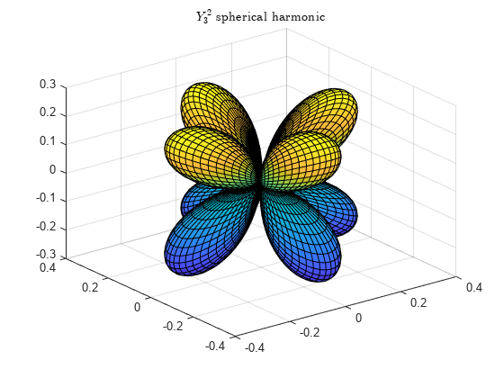
Spherical harmonics arise in the solution to Laplace's equation and are used to represent functions defined on the surface of a sphere. Use legendre to compute and visualize the spherical harmonic for .
The equation for spherical harmonics includes a term for the Legendre function, as well as a complex exponential:
First, create a grid of values to represent all combinations of (colatitude angle) and (azimuthal angle). Here, the colatitude ranges from 0 at the North Pole, to at the Equator, and to at the South Pole.
dx = pi/60;
col = 0:dx:pi;
az = 0:dx:2*pi;
[phi,theta] = meshgrid(az,col);
Calculate on the grid for .
l = 3;
Plm = legendre(l,cos(theta));
Since legendre computes the answer for all values of , Plm contains some extra function values. Extract the values for and discard the rest. Use the reshape function to orient the results as a matrix with the same size as phi and theta.
m = 2;
if l ~= 0
    Plm = reshape(Plm(m+1,:,:),size(phi));
end
Calculate the spherical harmonic values for .
a = (2*l+1)*factorial(l-m);
b = 4*pi*factorial(l+m);
C = sqrt(a/b);
Ylm = C .*Plm .*exp(1i*m*phi);
Convert the spherical coordinates to Cartesian coordinates. Here, becomes the latitude angle that ranges from at the North Pole, to 0 at the Equator, and to at the South Pole. Plot the spherical harmonic for using both the positive and negative real values.
[Xm,Ym,Zm] = sph2cart(phi, pi/2-theta, abs(real(Ylm)));
surf(Xm,Ym,Zm)
title('$Y_3^2$ spherical harmonic','interpreter','latex')
Input Arguments
Output Arguments
Limitations
The values of the unnormalized associated Legendre function overflow the range of
double-precision numbers for n > 150 and the range of single-precision
numbers for n > 28. This overflow results in Inf and
NaN values. For orders larger than these thresholds, consider using the
'sch' or 'norm' normalizations instead.
More About
Algorithms
legendre uses a three-term backward recursion relationship in
m. This recursion is on a version of the Schmidt seminormalized
associated Legendre functions , which are complex spherical harmonics. These functions are related to the
standard Abramowitz and Stegun [1] functions by
They are related to the Schmidt form by
References
[1] Abramowitz, M. and I. A. Stegun, Handbook of Mathematical Functions, Dover Publications, 1965, Ch.8.
[2] Jacobs, J. A., Geomagnetism, Academic Press, 1987, Ch.4.