Main Content

pchip

Piecewise Cubic Hermite Interpolating Polynomial (PCHIP)

Description

example

p = pchip(x,y,xq) returns a vector of interpolated values p corresponding to the query points in xq. The values of p are determined by shape-preserving piecewise cubic interpolation of x and y.

example

pp = pchip(x,y) returns a piecewise polynomial structure for use with ppval and the spline utility unmkpp.

Examples

collapse all

Compare the interpolation results produced by spline, pchip, and makima for two different data sets. These functions all perform different forms of piecewise cubic Hermite interpolation. Each function differs in how it computes the slopes of the interpolant, leading to different behaviors when the underlying data has flat areas or undulations.

Compare the interpolation results on sample data that connects flat regions. Create vectors of x values, function values at those points y, and query points xq. Compute interpolations at the query points using spline, pchip, and makima. Plot the interpolated function values at the query points for comparison.

x = -3:3; 
y = [-1 -1 -1 0 1 1 1]; 
xq1 = -3:.01:3;
p = pchip(x,y,xq1);
s = spline(x,y,xq1);
m = makima(x,y,xq1);
plot(x,y,'o',xq1,p,'-',xq1,s,'-.',xq1,m,'--')
legend('Sample Points','pchip','spline','makima','Location','SouthEast')

Figure contains an axes object. The axes object contains 4 objects of type line. One or more of the lines displays its values using only markers These objects represent Sample Points, pchip, spline, makima.

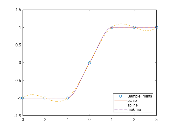
In this case, pchip and makima have similar behavior in that they avoid overshoots and can accurately connect the flat regions.

Perform a second comparison using an oscillatory sample function.

x = 0:15;
y = besselj(1,x);
xq2 = 0:0.01:15;
p = pchip(x,y,xq2);
s = spline(x,y,xq2);
m = makima(x,y,xq2);
plot(x,y,'o',xq2,p,'-',xq2,s,'-.',xq2,m,'--')
legend('Sample Points','pchip','spline','makima')

Figure contains an axes object. The axes object contains 4 objects of type line. One or more of the lines displays its values using only markers These objects represent Sample Points, pchip, spline, makima.

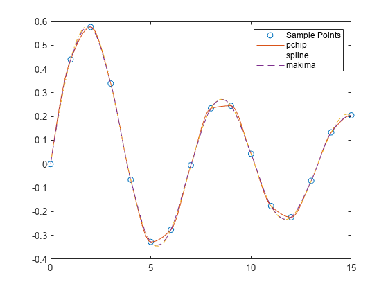
When the underlying function is oscillatory, spline and makima capture the movement between points better than pchip, which is aggressively flattened near local extrema.

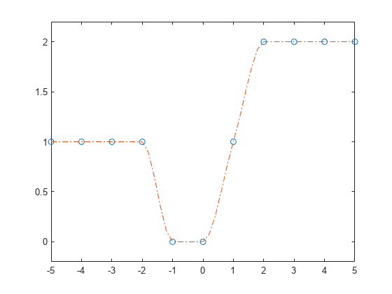
Create vectors for the x values and function values y, and then use pchip to construct a piecewise polynomial structure.

x = -5:5;
y = [1 1 1 1 0 0 1 2 2 2 2];
p = pchip(x,y);

Use the structure with ppval to evaluate the interpolation at several query points. Plot the results.

xq = -5:0.2:5;
pp = ppval(p,xq);
plot(x,y,'o',xq,pp,'-.')
ylim([-0.2 2.2])

Figure contains an axes object. The axes object contains 2 objects of type line. One or more of the lines displays its values using only markers

Input Arguments

collapse all

Sample points, specified as a vector. The vector x specifies the points at which the data y is given. The elements of x must be unique.

Data Types: single | double

Function values at sample points, specified as a numeric vector, matrix, or array. x and y must have the same length.

If y is a matrix or array, then the values in the last dimension, y(:,...,:,j), are taken as the values to match with x. In that case, the last dimension of y must be the same length as x.

Data Types: single | double

Query points, specified as a scalar, vector, matrix, or array. The points specified in xq are the x-coordinates for the interpolated function values yq computed by pchip.

Data Types: single | double

Output Arguments

collapse all

Interpolated values at query points, returned as a scalar, vector, matrix, or array. The size of p is related to the sizes of y and xq:

  • If y is a vector, then p has the same size as xq.

  • If y is an array of size Ny = size(y), then these conditions apply:

    • If xq is a scalar or vector, then size(p) returns [Ny(1:end-1) length(xq)].

    • If xq is an array, then size(p) returns [Ny(1:end-1) size(xq).

Piecewise polynomial, returned as a structure. Use this structure with the ppval function to evaluate the interpolating polynomials at one or more query points. The structure has these fields.

FieldDescription
form

'pp' for piecewise polynomial

breaks

Vector of length L+1 with strictly increasing elements that represent the start and end of each of L intervals

coefs

L-by-k matrix with each row coefs(i,:) containing the local coefficients of an order k polynomial on the ith interval, [breaks(i),breaks(i+1)]

pieces

Number of pieces, L

order

Order of the polynomials

dim

Dimensionality of target

Since the polynomial coefficients in coefs are local coefficients for each interval, you must subtract the lower endpoint of the corresponding knot interval to use the coefficients in a conventional polynomial equation. In other words, for the coefficients [a,b,c,d] on the interval [x1,x2], the corresponding polynomial is

f(x)=a(xx1)3+b(xx1)2+c(xx1)+d.

More About

collapse all

Shape-Preserving Piecewise Cubic Interpolation

pchip interpolates using a piecewise cubic polynomial P(x) with these properties:

  • On each subinterval xkxxk+1, the polynomial P(x) is a cubic Hermite interpolating polynomial for the given data points with specified derivatives (slopes) at the interpolation points.

  • P(x) interpolates y, that is, P(xj)=yj, and the first derivative dPdx is continuous. The second derivative d2Pdx2 is probably not continuous so jumps at the xj are possible.

  • The cubic interpolant P(x) is shape preserving. The slopes at the xj are chosen in such a way that P(x) preserves the shape of the data and respects monotonicity. Therefore, on intervals where the data is monotonic, so is P(x), and at points where the data has a local extremum, so does P(x).

Note

If y is a matrix, P(x) satisfies these properties for each row of y.

Tips

  • spline constructs S(x) in almost the same way pchip constructs P(x). However, spline chooses the slopes at the xj differently, namely to make even S(x) continuous. This difference has several effects:

    • spline produces a smoother result, such that S(x) is continuous.

    • spline produces a more accurate result if the data consists of values of a smooth function.

    • pchip has no overshoots and less oscillation if the data is not smooth.

    • pchip is less expensive to set up.

    • The two are equally expensive to evaluate.

References

[1] Fritsch, F. N. and R. E. Carlson. "Monotone Piecewise Cubic Interpolation." SIAM Journal on Numerical Analysis. Vol. 17, 1980, pp.238–246.

[2] Kahaner, David, Cleve Moler, Stephen Nash. Numerical Methods and Software. Upper Saddle River, NJ: Prentice Hall, 1988.

Extended Capabilities

Version History

Introduced before R2006a

See Also

| | |