narxnet
(To be removed) Nonlinear autoregressive neural network with external input
narxnet will be removed in a future release. For more information,
see Transition Legacy Neural Network Code to dlnetwork Workflows.
For advice on updating your code, see Version History.
Description
narxnet(
takes these arguments:inputDelays,feedbackDelays,hiddenSizes,feedbackMode,trainFcn)
Row vector of increasing 0 or positive input delays,
inputDelaysRow vector of increasing 0 or positive feedback delays,
feedbackDelaysRow vector of one or more hidden layer sizes,
hiddenSizesType of feedback,
feedbackModeBackpropagation training function,
trainFcn
and returns a NARX neural network.
NARX (Nonlinear autoregressive with external input) networks can learn to predict one time series given past values of the same time series, the feedback input, and another time series called the external (or exogenous) time series.
Examples
Train a nonlinear autoregressive with external input (NARX) neural network and predict on new time series data. Predicting a sequence of values in a time series is also known as multistep prediction. Closed-loop networks can perform multistep predictions. When external feedback is missing, closed-loop networks can continue to predict by using internal feedback. In NARX prediction, the future values of a time series are predicted from past values of that series, the feedback input, and an external time series.
Load the simple time series prediction data.
[X,T] = simpleseries_dataset;
Partition the data into training data XTrain and TTrain, and data for prediction XPredict. Use XPredict to perform prediction after you create the closed-loop network.
XTrain = X(1:80);
TTrain = T(1:80);
XPredict = X(81:100);
Create a NARX network. Define the input delays, feedback delays, and size of the hidden layers.
net = narxnet(1:2,1:2,10);
Prepare the time series data using preparets. This function automatically shifts input and target time series by the number of steps needed to fill the initial input and layer delay states.
[Xs,Xi,Ai,Ts] = preparets(net,XTrain,{},TTrain);A recommended practice is to fully create the network in an open loop, and then transform the network to a closed loop for multistep-ahead prediction. Then, the closed-loop network can predict as many future values as you want. If you simulate the neural network in closed-loop mode only, the network can perform as many predictions as the number of time steps in the input series.
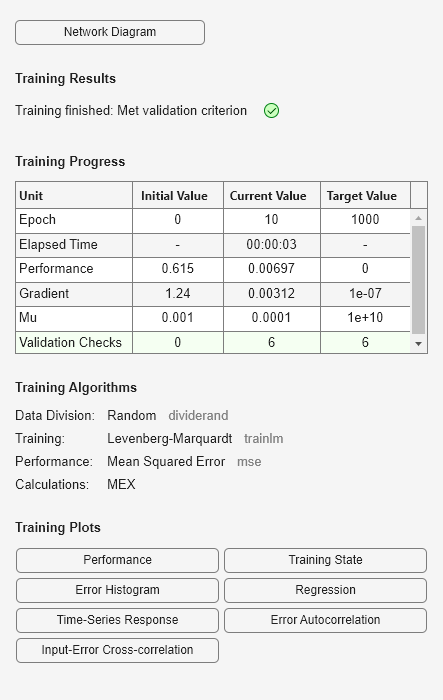
Train the NARX network. The train function trains the network in an open loop (series-parallel architecture), including the validation and testing steps.
net = train(net,Xs,Ts,Xi,Ai);
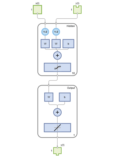
Display the trained network.
view(net)
Calculate the network output Y, final input states Xf, and final layer states Af of the open-loop network from the network input Xs, initial input states Xi, and initial layer states Ai.
[Y,Xf,Af] = net(Xs,Xi,Ai);
Calculate the network performance.
perf = perform(net,Ts,Y)
perf =
0.0153
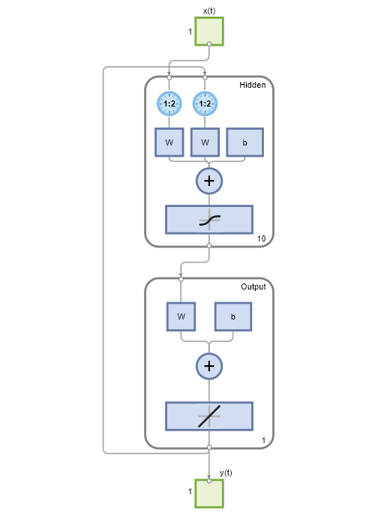
To predict the output for the next 20 time steps, first simulate the network in closed-loop mode. The final input states Xf and layer states Af of the open-loop network net become the initial input states Xic and layer states Aic of the closed-loop network netc.
[netc,Xic,Aic] = closeloop(net,Xf,Af);
Display the closed-loop network.
view(netc)
Run the prediction for 20 time steps ahead in closed-loop mode.
Yc = netc(XPredict,Xic,Aic)
Yc=1×20 cell array
    {[-0.0156]}    {[0.1133]}    {[-0.1472]}    {[-0.0706]}    {[0.0355]}    {[-0.2829]}    {[0.2047]}    {[-0.3809]}    {[-0.2836]}    {[0.1886]}    {[-0.1813]}    {[0.1373]}    {[0.2189]}    {[0.3122]}    {[0.2346]}    {[-0.0156]}    {[0.0724]}    {[0.3395]}    {[0.1940]}    {[0.0757]}