Calculate Gradients and Hessians Using Symbolic Math Toolbox
This example shows how to obtain faster and more robust solutions to nonlinear optimization problems using fmincon along with Symbolic Math Toolbox™ functions. If you have a Symbolic Math Toolbox license, you can easily calculate analytic gradients and Hessians for objective and constraint functions using these Symbolic Math Toolbox functions:
jacobian(Symbolic Math Toolbox) generates the gradient of a scalar function, and generates a matrix of the partial derivatives of a vector function. So, for example, you can obtain the Hessian matrix (the second derivatives of the objective function) by applyingjacobianto the gradient. This example shows how to usejacobianto generate symbolic gradients and Hessians of objective and constraint functions.matlabFunction(Symbolic Math Toolbox) generates either an anonymous function or a file that calculates the values of a symbolic expression. This example shows how to usematlabFunctionto generate files that evaluate the objective and constraint functions and their derivatives at arbitrary points.
Symbolic Math Toolbox functions have different syntaxes and structures compared to Optimization Toolbox™ functions. In particular, symbolic variables are real or complex scalars, whereas Optimization Toolbox functions pass vector arguments. So, you need to take several steps to symbolically generate the objective function, constraints, and all their requisite derivatives, in a form suitable for the interior-point algorithm of fmincon.
Problem-based optimization can calculate and use gradients automatically; see Automatic Differentiation in Optimization Toolbox. For a problem-based approach to this problem using automatic differentiation, see Constrained Electrostatic Nonlinear Optimization Using Optimization Variables.
Problem Description
Consider the electrostatics problem of placing 10 electrons in a conducting body. The electrons arrange themselves in a way that minimizes their total potential energy, subject to the constraint of lying inside the body. All the electrons are on the boundary of the body at a minimum. The electrons are indistinguishable, so no unique minimum exists for this problem (permuting the electrons in one solution gives another valid solution). This example is inspired by Dolan, Moré, and Munson [58].
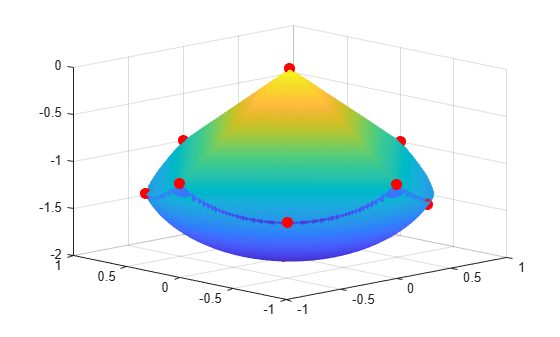
This example is a conducting body defined by the inequalities
.
This body looks like a pyramid on a sphere.
[X,Y] = meshgrid(-1:.01:1);
Z1 = -abs(X) - abs(Y);
Z2 = -1 - sqrt(1 - X.^2 - Y.^2);
Z2 = real(Z2);
W1 = Z1; W2 = Z2;
W1(Z1 < Z2) = nan; % Only plot points where Z1 > Z2
W2(Z1 < Z2) = nan; % Only plot points where Z1 > Z2
hand = figure; % Handle to the figure, for more plotting later
set(gcf,Color="w") % White background
surf(X,Y,W1,LineStyle="none");
hold on
surf(X,Y,W2,LineStyle="none");
view(-44,18)

A slight gap exists between the upper and lower surfaces of the figure. This gap is an artifact of the general plotting routine used to create the figure. The routine erases any rectangular patch on one surface that touches the other surface.
Create Variables
Generate a symbolic vector x as a 30-by-1 vector composed of real symbolic variables xij, with i between 1 and 10, and j between 1 and 3. These variables represent the three coordinates of electron i: xi1 corresponds to the coordinate, xi2 corresponds to the coordinate, and xi3 corresponds to the coordinate.
x = cell(3, 10);
for i = 1:10
    for j = 1:3
        x{j,i} = sprintf("x%d%d",i,j);
    end
end
x = x(:); % Now x is a 30-by-1 vector
x = sym(x, "real");
Display the vector x.
x
x =
Include Linear Constraints
Write the linear constraints
as a set of four linear inequalities for each electron:
xi3 - xi1 - xi2 ≤ 0
xi3 - xi1 + xi2 ≤ 0
xi3 + xi1 - xi2 ≤ 0
xi3 + xi1 + xi2 ≤ 0
So, this problem has a total of 40 linear inequalities.
Write the inequalities in a structured way.
B = [1,1,1;-1,1,1;1,-1,1;-1,-1,1];

A = zeros(40,30);
for i=1:10
    A(4*i-3:4*i,3*i-2:3*i) = B;
end

b = zeros(40,1);
You can see that A*x ≤ b represents the inequalities.
disp(A*x)
Create the Nonlinear Constraints and Their Gradients and Hessians
The nonlinear constraints are also structured.
.
Generate the constraints and their gradients and Hessians.
ineqnonlin = sym(zeros(1,10));
i = 1:10;
ineqnonlin = (x(3*i-2).^2 + x(3*i-1).^2 + (x(3*i)+1).^2 - 1).';

gradineqnonlin = jacobian(ineqnonlin,x).'; % .' performs transpose

hessineqnonlin = cell(1, 10);
for i = 1:10
    hessineqnonlin{i} = jacobian(gradineqnonlin(:,i),x);
end
The constraint vector ineqnonlin is a row vector, and the gradient of ineqnonlin(i) is represented in the ith column of the matrix gradineqnonlin. This form is correct, as described in Nonlinear Constraints.
The Hessian matrices, hessineqnonlin{1}, ..., hessineqnonlin{10}, are square and symmetric. This example stores them in a cell array, which is better than storing them in separate variables such as hessineqnonlin1, ..., hessineqnonlin10.
Use the .' syntax to transpose. The ' syntax means conjugate transpose, which has different symbolic derivatives.
Create the Objective Function and Its Gradient and Hessian
The objective function, potential energy, is the sum of the inverses of the distances between each electron pair.
.
The distance is the square root of the sum of the squares of the differences in the components of the vectors.
Calculate the energy (objective function) and its gradient and Hessian.
energy = sym(0);
for i = 1:3:25
    for j = i+3:3:28
        dist = x(i:i+2) - x(j:j+2);
        energy = energy + 1/sqrt(dist.'*dist);
    end
end

gradenergy = jacobian(energy,x).';

hessenergy = jacobian(gradenergy,x);
Create the Objective Function File
The objective function has two outputs, energy and gradenergy. Put both functions in one vector when calling matlabFunction to reduce the number of subexpressions that matlabFunction generates, and to return the gradient only when the calling function (fmincon in this case) requests both outputs. You can place the resulting files in any folder on the MATLAB path. In this case, place them in your current folder.
currdir = [pwd filesep]; % You might need to use currdir = pwd
filename = [currdir,'demoenergy.m'];
matlabFunction(energy,gradenergy,file=filename,vars={x});
matlabFunction returns energy as the first output and gradenergy as the second. The function also takes a single input vector {x} instead of a list of inputs x11, ..., x103.
The resulting file demoenergy.m contains the following lines or similar ones:
function [energy,gradenergy] = demoenergy(in1)
%DEMOENERGY
%   [ENERGY,GRADENERGY] = DEMOENERGY(IN1)
...
x101 = in1(28,:);
...
energy = et1+et2;
if nargout > 1
    ...
    gradenergy = [mt1;mt2;mt3;mt4];
end
This function has the correct form for an objective function with a gradient; see Writing Scalar Objective Functions.
Create the Constraint Function File
Generate the nonlinear constraint function, and put it in the correct format.
filename = [currdir,'democonstr.m'];
matlabFunction(ineqnonlin,[],gradineqnonlin,[],file=filename,vars={x},...
    outputs=["ineqnonlin","eqnonlin","gradineqnonlin","gradeqnonlin"]);
The resulting file democonstr.m contains the following lines or similar ones:
function [ineqnonlin,eqnonlin,gradineqnonlin,gradeqnonlin] = democonstr(in1)
%DEMOCONSTR
%    [INEQNONLIN,EQNONLIN,GRADINEQNONLIN,GRADEQNONLIN] = DEMOCONSTR(IN1)

...
x101 = in1(28,:);
...
ineqnonlin = [t2.^2+x11.^2+x12.^2-1.0,...
if nargout > 1
    eqnonlin = zeros(0,0);
end
if nargout > 2
    ...
    gradineqnonlin = reshape([mt1,mt2],30,10);
end
if nargout > 3
    gradeqnonlin = zeros(0,0);
end
end
This function has the correct form for a constraint function with a gradient; see Nonlinear Constraints.
Generate the Hessian Files
To generate the Hessian of the Lagrangian for the problem, first generate files for the energy Hessian and the constraint Hessians.
The Hessian of the objective function, hessenergy, is a large symbolic expression containing over 150,000 symbols, as shown by evaluating size(char(hessenergy)). So, running matlabFunction(hessenergy) takes a substantial amount of time.
Generate the file hessenergy.m.
filename = [currdir,'hessenergy.m'];
matlabFunction(hessenergy,file=filename,vars={x});
In contrast, the Hessians of the constraint functions are small and fast to compute.
for i = 1:10
    ii = num2str(i);
    thename = ['hessc',ii];
    filename = [currdir,thename,'.m'];
    matlabFunction(hessineqnonlin{i},file=filename,vars={x});
end
After generating all the files for the objective and constraints, put them together with the appropriate Lagrange multipliers in the helper function hessfinal.m, whose code appears at the end of this example.
Run the Optimization
Start the optimization with the electrons distributed randomly on a sphere of radius 1/2 centered at [0,0,–1].
rng default % For reproducibility
Xinitial = randn(3,10); % Columns are normal 3-D vectors
for j=1:10
    Xinitial(:,j) = Xinitial(:,j)/norm(Xinitial(:,j))/2;
    % This normalizes to a 1/2-sphere
end
Xinitial(3,:) = Xinitial(3,:) - 1; % Center at [0,0,-1]
Xinitial = Xinitial(:); % Convert to a column vector
Set options to use the interior-point algorithm, and to use gradients and the Hessian.
options = optimoptions(@fmincon,Algorithm="interior-point",SpecifyObjectiveGradient=true,...
    SpecifyConstraintGradient=true,HessianFcn=@hessfinal,Display="final");
Call fmincon.
[xfinal,fval,exitflag,output] = fmincon(@demoenergy,Xinitial,...
A,b,[],[],[],[],@democonstr,options);
Local minimum found that satisfies the constraints. Optimization completed because the objective function is non-decreasing in feasible directions, to within the value of the optimality tolerance, and constraints are satisfied to within the value of the constraint tolerance. <stopping criteria details>
View the objective function value, exit flag, number of iterations, and number of function evaluations.
disp(fval)
34.1365
disp(exitflag)
1
disp(output.iterations)
19
disp(output.funcCount)
28
Even though the initial positions of the electrons are random, the final positions are nearly symmetric.
for i = 1:10
plot3(xfinal(3*i-2),xfinal(3*i-1),xfinal(3*i),"r.",MarkerSize=25);
end
To examine the entire 3-D geometry, rotate the figure.
rotate3d
figure(hand)
Compare to Optimization Without Gradients and Hessians
The use of gradients and Hessians makes the optimization run faster and more accurately. To compare the same optimization using no gradient or Hessian information, set options to not use gradients and Hessians.
options = optimoptions(@fmincon,Algorithm="interior-point",...
    Display="final");
[xfinal2,fval2,exitflag2,output2] = fmincon(@demoenergy,Xinitial,...
A,b,[],[],[],[],@democonstr,options);
Feasible point with lower objective function value found, but optimality criteria not satisfied. See output.bestfeasible..


Local minimum found that satisfies the constraints.

Optimization completed because the objective function is non-decreasing in
feasible directions, to within the value of the optimality tolerance,
and constraints are satisfied to within the value of the constraint tolerance.

<stopping criteria details>
View the objective function value, exit flag, number of iterations, and number of function evaluations.
disp(fval2)
34.1365
disp(exitflag2)
1
disp(output2.iterations)
76
disp(output2.funcCount)
2401
Compare the number of iterations and number of function evaluations with and without derivative information.
tbl = table([output.iterations;output2.iterations],[output.funcCount;output2.funcCount],...
RowNames=["With Derivatives","Without Derivatives"],VariableNames=["Iterations","Fevals"])
tbl=2×2 table
                           Iterations    Fevals
                           __________    ______

    With Derivatives           19           28
    Without Derivatives        76         2401
Clear the Symbolic Variable Assumptions
The symbolic variables in this example have the assumption that they are real in the symbolic engine workspace. Deleting the variables does not clear this assumption from the symbolic engine workspace. Clear the variable assumptions by using syms.
syms xVerify that the assumptions are empty.
assumptions(x)
ans =

Empty sym: 1-by-0
Helper Function
The following code creates the hessfinal helper function.
function H = hessfinal(X,lambda)
%
% Call the function hessenergy to start
H = hessenergy(X);

% Add the Lagrange multipliers * the constraint Hessians
H = H + hessc1(X) * lambda.ineqnonlin(1);
H = H + hessc2(X) * lambda.ineqnonlin(2);
H = H + hessc3(X) * lambda.ineqnonlin(3);
H = H + hessc4(X) * lambda.ineqnonlin(4);
H = H + hessc5(X) * lambda.ineqnonlin(5);
H = H + hessc6(X) * lambda.ineqnonlin(6);
H = H + hessc7(X) * lambda.ineqnonlin(7);
H = H + hessc8(X) * lambda.ineqnonlin(8);
H = H + hessc9(X) * lambda.ineqnonlin(9);
H = H + hessc10(X) * lambda.ineqnonlin(10);
end