statelevels
State-level estimation for bilevel waveform with histogram method
Syntax
Description
levels = statelevels(x)x using the histogram method. For more information, see
Algorithms.
statelevels(___) displays a plot of the
signal and the corresponding histogram.
Examples
Display State Levels and Subhistograms
Estimate the low- and high-state levels of 2.3 V underdamped clock data. Plot the data with the estimated state levels and subhistograms.
load("clockex.mat","x")

statelevels(x)

ans = 1×2

    0.0027    2.3068
State Levels with 100 Bins and Modes of Subhistograms
Estimate the low- and high-state levels of 2.3 V underdamped clock data sampled at 4 MHz.
Use the default number of bins and modes of the subhistograms to estimate the state levels.
load("clockex.mat","x","t")
levs = statelevels(x)
levs = 1×2

    0.0027    2.3068
Plot the clock data with the lines indicating the estimated low- and high-state levels.
statelevels(x)

ans = 1×2

    0.0027    2.3068
State Levels Using Means of Subhistograms
Estimate the low- and high-state levels of 2.3 V underdamped clock data sampled at 4 MHz.
Use the default number of bins and means of the subhistograms to estimate the state levels. Plot the clock data with the lines indicating the estimated low- and high-state levels.
load("clockex.mat","x","t")

statelevels(x,1e3,'mean')

ans = 1×2

   -0.0014    2.3014
Histogram Counts and Histogram Bin Centers
Estimate the low- and high-state levels of 2.3 V underdamped clock data sampled at 4 MHz. Return the histogram counts and histogram bin centers used in the histogram method. Use four bins.
load("clockex.mat","x","t")
[levs,histog,bilevs] = statelevels(x,4)
levs = 1×2

    0.2427    2.0428
histog = 4×1

    50
     0
     0
    50
bilevs = 4×1

    0.2427
    0.8427
    1.4428
    2.0428
Plot the waveform and annotate the levels.
statelevels(x,4)

ans = 1×2

    0.2427    2.0428
Input Arguments
Output Arguments
More About
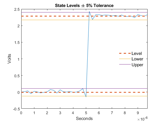
State-Level Tolerances
You can specify lower- and upper-state boundaries for each state level. Define the boundaries as the state level plus or minus a scalar multiple of the difference between the high state and the low state. To provide a useful tolerance region, specify the scalar as a small number such as 2/100 or 3/100. In general, the  region for the low state is defined as
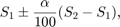
where  is the low-state level and
  is the high-state level. Replace the first term in the equation with to obtain the tolerance region for the high state.
This figure shows lower and upper 5% state boundaries (tolerance regions) for a positive-polarity bilevel waveform. The thick dashed lines indicate the estimated state levels.
Algorithms
statelevels uses the histogram method to estimate the states of a bilevel
waveform. The histogram method is described in [1]. The steps of this
method are:
Determine the maximum and minimum amplitudes and amplitude range of the data.
For the specified number of histogram bins, determine the bin width, which is the ratio of the amplitude range to the number of bins.
Sort the data values into the histogram bins.
Identify the lowest-indexed histogram bin, , and highest-indexed histogram bin, ihigh, with nonzero counts.
Divide the histogram into two subhistograms:
The indices of the lower histogram bins are .
The indices of the upper histogram bins are .
Compute the state levels by determining the mode or mean of the lower and upper histograms.
References
[1] IEEE® Standard on Transitions, Pulses, and Related Waveforms, IEEE Standard 181, 2003, pp. 15–17.
Extended Capabilities
Version History
Introduced in R2012a
See Also
midcross | overshoot | risetime | undershoot
You can also select a web site from the following list:
Americas
- América Latina (Español)
- Canada (English)
- United States (English)
Europe
- Belgium (English)
- Denmark (English)
- Deutschland (Deutsch)
- España (Español)
- Finland (English)
- France (Français)
- Ireland (English)
- Italia (Italiano)
- Luxembourg (English)
- Netherlands (English)
- Norway (English)
- Österreich (Deutsch)
- Portugal (English)
- Sweden (English)
- Switzerland
- United Kingdom (English)