fitrtree

Fit binary decision tree for regression

Syntax

Mdl = fitrtree(Tbl,ResponseVarName)

Mdl = fitrtree(Tbl,formula)

Mdl = fitrtree(Tbl,Y)

Mdl = fitrtree(X,Y)

Mdl = fitrtree(___,Name=Value)

[Mdl,AggregateOptimizationResults] = fitrtree(___)

Description

Mdl = fitrtree(Tbl,ResponseVarName) returns a regression tree based on the input variables (also known as predictors, features, or attributes) in the table Tbl and the output (response) contained in Tbl.ResponseVarName. The returned Mdl is a binary tree where each branching node is split based on the values of a column of Tbl.

Mdl = fitrtree(Tbl,formula) returns a regression tree based on the input variables contained in the table Tbl. The input formula is an explanatory model of the response and a subset of predictor variables in Tbl used to fit Mdl.

Mdl = fitrtree(Tbl,Y) returns a regression tree based on the input variables contained in the table Tbl and the output in vector Y.

Mdl = fitrtree(X,Y) returns a regression tree based on the input variables X and the output Y. The returned Mdl is a binary tree where each branching node is split based on the values of a column of X.

Mdl = fitrtree(___,Name=Value) specifies options using one or more name-value arguments in addition to any of the input argument combinations in previous syntaxes. For example, you can specify observation weights or train a cross-validated model.

[Mdl,AggregateOptimizationResults] = fitrtree(___) also returns AggregateOptimizationResults, which contains hyperparameter optimization results when you specify the OptimizeHyperparameters and HyperparameterOptimizationOptions name-value arguments. You must also specify the ConstraintType and ConstraintBounds options of HyperparameterOptimizationOptions. You can use this syntax to optimize on compact model size instead of cross-validation loss, and to perform a set of multiple optimization problems that have the same options but different constraint bounds.

Note

For a list of supported syntaxes when the input variables are tall arrays, see Tall Arrays.

Examples

Construct Regression Tree

Load the sample data.

load carsmall

Construct a regression tree using the sample data. The response variable is miles per gallon, MPG.

tree = fitrtree([Weight, Cylinders],MPG,...
                'CategoricalPredictors',2,'MinParentSize',20,...
                'PredictorNames',{'W','C'})

tree = 
  RegressionTree
           PredictorNames: {'W'  'C'}
             ResponseName: 'Y'
    CategoricalPredictors: 2
        ResponseTransform: 'none'
          NumObservations: 94


  Properties, Methods

Predict the mileage of 4,000-pound cars with 4, 6, and 8 cylinders.

MPG4Kpred = predict(tree,[4000 4; 4000 6; 4000 8])

MPG4Kpred = 3×1

   19.2778
   19.2778
   14.3889

Control Regression Tree Depth

fitrtree grows deep decision trees by default. You can grow shallower trees to reduce model complexity or computation time. To control the depth of trees, use the 'MaxNumSplits', 'MinLeafSize', or 'MinParentSize' name-value pair arguments.

Load the carsmall data set. Consider Displacement, Horsepower, and Weight as predictors of the response MPG.

load carsmall
X = [Displacement Horsepower Weight];

The default values of the tree-depth controllers for growing regression trees are:

• n - 1 for MaxNumSplits. n is the training sample size.

• 1 for MinLeafSize.

• 10 for MinParentSize.

These default values tend to grow deep trees for large training sample sizes.

Train a regression tree using the default values for tree-depth control. Cross-validate the model using 10-fold cross-validation.

rng(1); % For reproducibility
MdlDefault = fitrtree(X,MPG,'CrossVal','on');

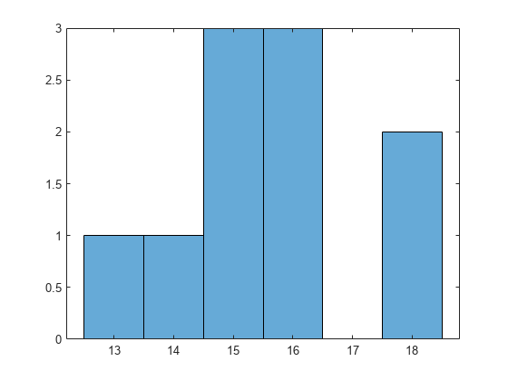
Draw a histogram of the number of imposed splits on the trees. The number of imposed splits is one less than the number of leaves. Also, view one of the trees.

numBranches = @(x)sum(x.IsBranch);
mdlDefaultNumSplits = cellfun(numBranches, MdlDefault.Trained);

figure;
histogram(mdlDefaultNumSplits)

view(MdlDefault.Trained{1},'Mode','graph')

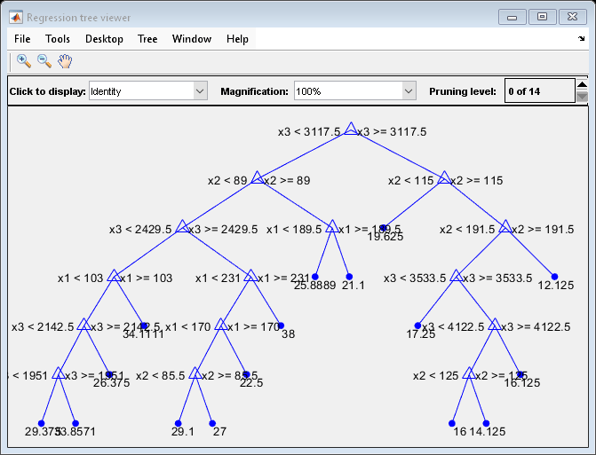
The average number of splits is between 14 and 15.

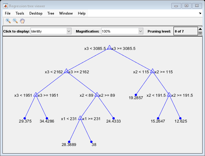
Suppose that you want a regression tree that is not as complex (deep) as the ones trained using the default number of splits. Train another regression tree, but set the maximum number of splits at 7, which is about half the mean number of splits from the default regression tree. Cross-validate the model using 10-fold cross-validation.

Mdl7 = fitrtree(X,MPG,'MaxNumSplits',7,'CrossVal','on');
view(Mdl7.Trained{1},'Mode','graph')

Compare the cross-validation mean squared errors (MSEs) of the models.

mseDefault = kfoldLoss(MdlDefault)

mseDefault = 
25.7383

mse7 = kfoldLoss(Mdl7)

mse7 = 
26.5748

Mdl7 is much less complex and performs only slightly worse than MdlDefault.

Optimize Regression Tree

Automatically optimize hyperparameters of a regression tree model by using fitrtree.

Load the carsmall data set.

load carsmall

Specify Horsepower and Weight as the predictor variables (X) and MPG as the response variable (Y).

X = [Horsepower Weight];
Y = MPG;

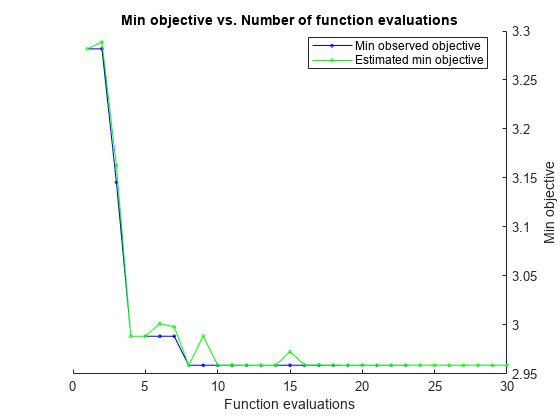
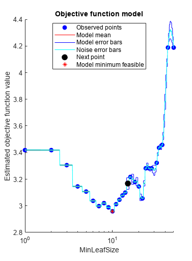
Find hyperparameters that minimize the 5-fold cross-validation loss by using automatic hyperparameter optimization. For reproducibility, set the random seed and use the "expected-improvement-plus" acquisition function.

rng(0,"twister")
hpoOptions = hyperparameterOptimizationOptions(AcquisitionFunctionName="expected-improvement-plus");
Mdl = fitrtree(X,Y,OptimizeHyperparameters="auto", ...
    HyperparameterOptimizationOptions=hpoOptions)

|======================================================================================|
| Iter | Eval   | Objective:  | Objective   | BestSoFar   | BestSoFar   |  MinLeafSize |
|      | result | log(1+loss) | runtime     | (observed)  | (estim.)    |              |
|======================================================================================|
|    1 | Best   |      3.2818 |     0.22434 |      3.2818 |      3.2818 |           28 |
|    2 | Accept |      3.4183 |    0.041183 |      3.2818 |      3.2888 |            1 |
|    3 | Best   |      3.1457 |    0.033462 |      3.1457 |      3.1628 |            4 |
|    4 | Best   |      2.9885 |     0.03489 |      2.9885 |      2.9885 |            9 |
|    5 | Accept |      2.9978 |    0.036753 |      2.9885 |      2.9885 |            7 |
|    6 | Accept |      3.0203 |    0.027979 |      2.9885 |      3.0013 |            8 |
|    7 | Accept |      2.9885 |    0.036313 |      2.9885 |      2.9981 |            9 |
|    8 | Best   |      2.9589 |    0.032478 |      2.9589 |      2.9589 |           10 |
|    9 | Accept |       3.078 |    0.031265 |      2.9589 |      2.9888 |           13 |
|   10 | Accept |      4.1881 |    0.034638 |      2.9589 |      2.9592 |           50 |
|   11 | Accept |      3.4182 |    0.050318 |      2.9589 |      2.9592 |            2 |
|   12 | Accept |      3.0376 |    0.024148 |      2.9589 |      2.9591 |            6 |
|   13 | Accept |      3.1453 |    0.022925 |      2.9589 |      2.9591 |           20 |
|   14 | Accept |      2.9589 |    0.031924 |      2.9589 |       2.959 |           10 |
|   15 | Accept |      3.0123 |    0.026502 |      2.9589 |      2.9728 |           11 |
|   16 | Accept |      2.9589 |    0.025416 |      2.9589 |      2.9593 |           10 |
|   17 | Accept |      3.3055 |    0.029169 |      2.9589 |      2.9593 |            3 |
|   18 | Accept |      2.9589 |    0.023451 |      2.9589 |      2.9592 |           10 |
|   19 | Accept |      3.4577 |    0.026011 |      2.9589 |      2.9591 |           37 |
|   20 | Accept |      3.2166 |    0.041208 |      2.9589 |       2.959 |           16 |
|======================================================================================|
| Iter | Eval   | Objective:  | Objective   | BestSoFar   | BestSoFar   |  MinLeafSize |
|      | result | log(1+loss) | runtime     | (observed)  | (estim.)    |              |
|======================================================================================|
|   21 | Accept |      3.1073 |    0.026594 |      2.9589 |      2.9591 |            5 |
|   22 | Accept |      3.2818 |    0.022941 |      2.9589 |       2.959 |           24 |
|   23 | Accept |      3.3226 |    0.023155 |      2.9589 |       2.959 |           32 |
|   24 | Accept |      4.1881 |    0.024017 |      2.9589 |      2.9589 |           43 |
|   25 | Accept |      3.1789 |    0.026557 |      2.9589 |      2.9589 |           18 |
|   26 | Accept |      3.0992 |    0.042702 |      2.9589 |      2.9589 |           14 |
|   27 | Accept |      3.0556 |    0.024676 |      2.9589 |      2.9589 |           22 |
|   28 | Accept |      3.0522 |    0.034223 |      2.9589 |      2.9589 |           12 |
|   29 | Accept |      3.2818 |    0.034522 |      2.9589 |      2.9589 |           26 |
|   30 | Accept |      3.4361 |    0.031322 |      2.9589 |      2.9589 |           34 |

__________________________________________________________
Optimization completed.
MaxObjectiveEvaluations of 30 reached.
Total function evaluations: 30
Total elapsed time: 20.0495 seconds
Total objective function evaluation time: 1.1251

Best observed feasible point:
    MinLeafSize
    ___________

        10     

Observed objective function value = 2.9589
Estimated objective function value = 2.9589
Function evaluation time = 0.032478

Best estimated feasible point (according to models):
    MinLeafSize
    ___________

        10     

Estimated objective function value = 2.9589
Estimated function evaluation time = 0.032458

Mdl = 
  RegressionTree
                         ResponseName: 'Y'
                CategoricalPredictors: []
                    ResponseTransform: 'none'
                      NumObservations: 94
    HyperparameterOptimizationResults: [1×1 classreg.learning.paramoptim.SupervisedLearningBayesianOptimization]


  Properties, Methods

The trained model Mdl corresponds to the best estimated feasible point and uses the same MinLeafSize hyperparameter value.

Find the hyperparameter value used to train Mdl by using the bestPoint function. By default, bestPoint uses the same best point criterion used by fitrtree during the hyperparameter optimization ("min-visited-upper-confidence-interval"). In general, fit functions determine the best hyperparameter values based on the "min-visited-upper-confidence-interval" criterion (instead of the "min-observed" criterion) to avoid overfitting to noise in the data set.

bestEstimatedPoint = bestPoint(Mdl.HyperparameterOptimizationResults)

bestEstimatedPoint=table
    MinLeafSize
    ___________

        10     

Verify that the result matches the property of Mdl.

Mdl.ModelParameters.MinLeaf

ans = 
10

Unbiased Predictor Importance Estimates

Load the carsmall data set. Consider a model that predicts the mean fuel economy of a car given its acceleration, number of cylinders, engine displacement, horsepower, manufacturer, model year, and weight. Consider Cylinders, Mfg, and Model_Year as categorical variables.

load carsmall
Cylinders = categorical(Cylinders);
Mfg = categorical(cellstr(Mfg));
Model_Year = categorical(Model_Year);
X = table(Acceleration,Cylinders,Displacement,Horsepower,Mfg, ...
    Model_Year,Weight,MPG);

Display the number of categories represented in the categorical variables.

numCylinders = numel(categories(Cylinders))

numCylinders = 
3

numMfg = numel(categories(Mfg))

numMfg = 
28

numModelYear = numel(categories(Model_Year))

numModelYear = 
3

Because there are 3 categories only in Cylinders and Model_Year, the standard CART, predictor-splitting algorithm prefers splitting a continuous predictor over these two variables.

Train a regression tree using the entire data set. To grow unbiased trees, specify usage of the curvature test for splitting predictors. Because there are missing values in the data, specify usage of surrogate splits.

Mdl = fitrtree(X,"MPG",PredictorSelection="curvature",Surrogate="on");

Estimate predictor importance values by summing changes in the risk due to splits on every predictor and dividing the sum by the number of branch nodes. Compare the estimates using a bar graph.

imp = predictorImportance(Mdl);

figure
bar(imp)
title("Predictor Importance Estimates")
ylabel("Estimates")
xlabel("Predictors")
h = gca;
h.XTickLabel = Mdl.PredictorNames;
h.XTickLabelRotation = 45;
h.TickLabelInterpreter = "none";

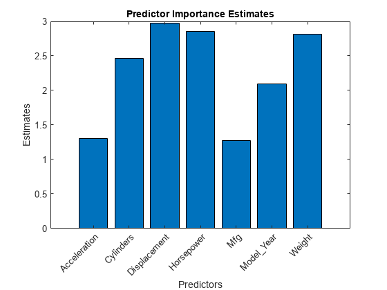
In this case, Displacement is the most important predictor, followed by Horsepower.

Control Maximum Tree Depth on Tall Array

fitrtree grows deep decision trees by default. Build a shallower tree that requires fewer passes through a tall array. Use the 'MaxDepth' name-value pair argument to control the maximum tree depth.

When you perform calculations on tall arrays, MATLAB® uses either a parallel pool (default if you have Parallel Computing Toolbox™) or the local MATLAB session. If you want to run the example using the local MATLAB session when you have Parallel Computing Toolbox, you can change the global execution environment by using the mapreducer function.

Load the carsmall data set. Consider Displacement, Horsepower, and Weight as predictors of the response MPG.

load carsmall
X = [Displacement Horsepower Weight];

Convert the in-memory arrays X and MPG to tall arrays.

tx = tall(X);

Starting parallel pool (parpool) using the 'local' profile ...
Connected to the parallel pool (number of workers: 6).

ty = tall(MPG);

Grow a regression tree using all observations. Allow the tree to grow to the maximum possible depth.

For reproducibility, set the seeds of the random number generators using rng and tallrng. The results can vary depending on the number of workers and the execution environment for the tall arrays. For details, see Control Where Your Code Runs.

rng('default') 
tallrng('default')
Mdl = fitrtree(tx,ty);

Evaluating tall expression using the Parallel Pool 'local':
- Pass 1 of 2: Completed in 4.1 sec
- Pass 2 of 2: Completed in 0.71 sec
Evaluation completed in 6.7 sec
Evaluating tall expression using the Parallel Pool 'local':
- Pass 1 of 7: Completed in 1.4 sec
- Pass 2 of 7: Completed in 0.29 sec
- Pass 3 of 7: Completed in 1.5 sec
- Pass 4 of 7: Completed in 3.3 sec
- Pass 5 of 7: Completed in 0.63 sec
- Pass 6 of 7: Completed in 1.2 sec
- Pass 7 of 7: Completed in 2.6 sec
Evaluation completed in 12 sec
Evaluating tall expression using the Parallel Pool 'local':
- Pass 1 of 7: Completed in 0.36 sec
- Pass 2 of 7: Completed in 0.27 sec
- Pass 3 of 7: Completed in 0.85 sec
- Pass 4 of 7: Completed in 2 sec
- Pass 5 of 7: Completed in 0.55 sec
- Pass 6 of 7: Completed in 0.92 sec
- Pass 7 of 7: Completed in 1.6 sec
Evaluation completed in 7.4 sec
Evaluating tall expression using the Parallel Pool 'local':
- Pass 1 of 7: Completed in 0.32 sec
- Pass 2 of 7: Completed in 0.29 sec
- Pass 3 of 7: Completed in 0.89 sec
- Pass 4 of 7: Completed in 1.9 sec
- Pass 5 of 7: Completed in 0.83 sec
- Pass 6 of 7: Completed in 1.2 sec
- Pass 7 of 7: Completed in 2.4 sec
Evaluation completed in 9 sec
Evaluating tall expression using the Parallel Pool 'local':
- Pass 1 of 7: Completed in 0.33 sec
- Pass 2 of 7: Completed in 0.28 sec
- Pass 3 of 7: Completed in 0.89 sec
- Pass 4 of 7: Completed in 2.4 sec
- Pass 5 of 7: Completed in 0.76 sec
- Pass 6 of 7: Completed in 1 sec
- Pass 7 of 7: Completed in 1.7 sec
Evaluation completed in 8.3 sec
Evaluating tall expression using the Parallel Pool 'local':
- Pass 1 of 7: Completed in 0.34 sec
- Pass 2 of 7: Completed in 0.26 sec
- Pass 3 of 7: Completed in 0.81 sec
- Pass 4 of 7: Completed in 1.7 sec
- Pass 5 of 7: Completed in 0.56 sec
- Pass 6 of 7: Completed in 1 sec
- Pass 7 of 7: Completed in 1.9 sec
Evaluation completed in 7.4 sec
Evaluating tall expression using the Parallel Pool 'local':
- Pass 1 of 7: Completed in 0.35 sec
- Pass 2 of 7: Completed in 0.28 sec
- Pass 3 of 7: Completed in 0.81 sec
- Pass 4 of 7: Completed in 1.8 sec
- Pass 5 of 7: Completed in 0.76 sec
- Pass 6 of 7: Completed in 0.96 sec
- Pass 7 of 7: Completed in 2.2 sec
Evaluation completed in 8 sec
Evaluating tall expression using the Parallel Pool 'local':
- Pass 1 of 7: Completed in 0.35 sec
- Pass 2 of 7: Completed in 0.32 sec
- Pass 3 of 7: Completed in 0.92 sec
- Pass 4 of 7: Completed in 1.9 sec
- Pass 5 of 7: Completed in 1 sec
- Pass 6 of 7: Completed in 1.5 sec
- Pass 7 of 7: Completed in 2.1 sec
Evaluation completed in 9.2 sec
Evaluating tall expression using the Parallel Pool 'local':
- Pass 1 of 7: Completed in 0.33 sec
- Pass 2 of 7: Completed in 0.28 sec
- Pass 3 of 7: Completed in 0.82 sec
- Pass 4 of 7: Completed in 1.4 sec
- Pass 5 of 7: Completed in 0.61 sec
- Pass 6 of 7: Completed in 0.93 sec
- Pass 7 of 7: Completed in 1.5 sec
Evaluation completed in 6.6 sec

View the trained tree Mdl.

view(Mdl,'Mode','graph')

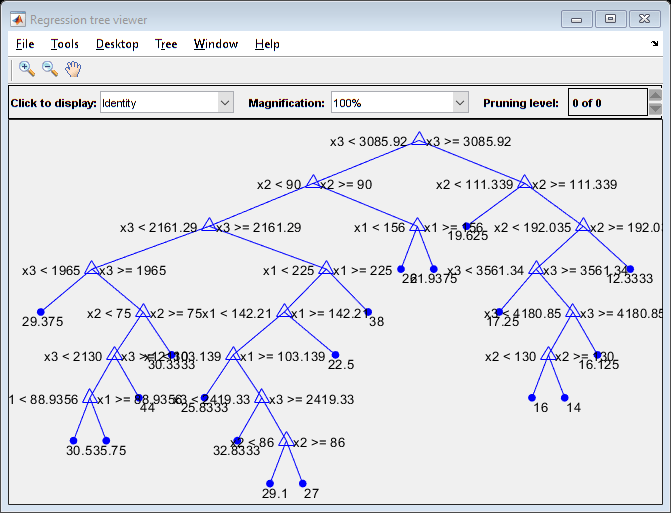
Mdl is a tree of depth 8.

Estimate the in-sample mean squared error.

MSE_Mdl = gather(loss(Mdl,tx,ty))

Evaluating tall expression using the Parallel Pool 'local':
- Pass 1 of 1: Completed in 1.6 sec
Evaluation completed in 1.9 sec

MSE_Mdl = 4.9078

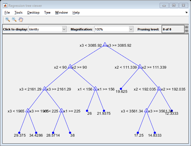
Grow a regression tree using all observations. Limit the tree depth by specifying a maximum tree depth of 4.

Mdl2 = fitrtree(tx,ty,'MaxDepth',4);

Evaluating tall expression using the Parallel Pool 'local':
- Pass 1 of 2: Completed in 0.27 sec
- Pass 2 of 2: Completed in 0.28 sec
Evaluation completed in 0.84 sec
Evaluating tall expression using the Parallel Pool 'local':
- Pass 1 of 7: Completed in 0.36 sec
- Pass 2 of 7: Completed in 0.3 sec
- Pass 3 of 7: Completed in 0.95 sec
- Pass 4 of 7: Completed in 1.6 sec
- Pass 5 of 7: Completed in 0.55 sec
- Pass 6 of 7: Completed in 0.93 sec
- Pass 7 of 7: Completed in 1.5 sec
Evaluation completed in 7 sec
Evaluating tall expression using the Parallel Pool 'local':
- Pass 1 of 7: Completed in 0.34 sec
- Pass 2 of 7: Completed in 0.3 sec
- Pass 3 of 7: Completed in 0.95 sec
- Pass 4 of 7: Completed in 1.7 sec
- Pass 5 of 7: Completed in 0.57 sec
- Pass 6 of 7: Completed in 0.94 sec
- Pass 7 of 7: Completed in 1.8 sec
Evaluation completed in 7.7 sec
Evaluating tall expression using the Parallel Pool 'local':
- Pass 1 of 7: Completed in 0.34 sec
- Pass 2 of 7: Completed in 0.3 sec
- Pass 3 of 7: Completed in 0.87 sec
- Pass 4 of 7: Completed in 1.5 sec
- Pass 5 of 7: Completed in 0.57 sec
- Pass 6 of 7: Completed in 0.81 sec
- Pass 7 of 7: Completed in 1.7 sec
Evaluation completed in 6.9 sec
Evaluating tall expression using the Parallel Pool 'local':
- Pass 1 of 7: Completed in 0.32 sec
- Pass 2 of 7: Completed in 0.27 sec
- Pass 3 of 7: Completed in 0.85 sec
- Pass 4 of 7: Completed in 1.6 sec
- Pass 5 of 7: Completed in 0.63 sec
- Pass 6 of 7: Completed in 0.9 sec
- Pass 7 of 7: Completed in 1.6 sec
Evaluation completed in 7 sec

View the trained tree Mdl2.

view(Mdl2,'Mode','graph')

Estimate the in-sample mean squared error.

MSE_Mdl2 = gather(loss(Mdl2,tx,ty))

Evaluating tall expression using the Parallel Pool 'local':
- Pass 1 of 1: Completed in 0.73 sec
Evaluation completed in 1 sec

MSE_Mdl2 = 9.3903

Mdl2 is a less complex tree with a depth of 4 and an in-sample mean squared error that is higher than the mean squared error of Mdl.

Input Arguments

Tbl — Sample data

table

Sample data used to train the model, specified as a table. Each row of Tbl corresponds to one observation, and each column corresponds to one predictor variable. Optionally, Tbl can contain one additional column for the response variable. Multicolumn variables and cell arrays other than cell arrays of character vectors are not allowed.

• If Tbl contains the response variable, and you want to use all remaining variables in Tbl as predictors, then specify the response variable by using ResponseVarName.

• If Tbl contains the response variable, and you want to use only a subset of the remaining variables in Tbl as predictors, then specify a formula by using formula.

• If Tbl does not contain the response variable, then specify a response variable by using Y. The length of the response variable and the number of rows in Tbl must be equal.

ResponseVarName — Response variable name

name of variable in Tbl

Response variable name, specified as the name of a variable in Tbl. The response variable must be a numeric vector.

You must specify ResponseVarName as a character vector or string scalar. For example, if Tbl stores the response variable Y as Tbl.Y, then specify it as "Y". Otherwise, the software treats all columns of Tbl, including Y, as predictors when training the model.

Data Types: char | string

formula — Explanatory model of response variable and subset of predictor variables

character vector | string scalar

Explanatory model of the response variable and a subset of the predictor variables, specified as a character vector or string scalar in the form "Y~x1+x2+x3". In this form, Y represents the response variable, and x1, x2, and x3 represent the predictor variables.

To specify a subset of variables in Tbl as predictors for training the model, use a formula. If you specify a formula, then the software does not use any variables in Tbl that do not appear in formula.

The variable names in the formula must be both variable names in Tbl (Tbl.Properties.VariableNames) and valid MATLAB^® identifiers. You can verify the variable names in Tbl by using the isvarname function. If the variable names are not valid, then you can convert them by using the matlab.lang.makeValidName function.

Data Types: char | string

Y — Response data

numeric column vector

Response data, specified as a numeric column vector with the same number of rows as X. Each entry in Y is the response to the data in the corresponding row of X.

The software considers NaN values in Y to be missing values. fitrtree does not use observations with missing values for Y in the fit.

Data Types: single | double

X — Predictor data

numeric matrix

Predictor data, specified as a numeric matrix. Each column of X represents one variable, and each row represents one observation.

fitrtree considers NaN values in X as missing values. fitrtree does not use observations with all missing values for X in the fit. fitrtree uses observations with some missing values for X to find splits on variables for which these observations have valid values.

Data Types: single | double

Name-Value Arguments

Specify optional pairs of arguments as Name1=Value1,...,NameN=ValueN, where Name is the argument name and Value is the corresponding value. Name-value arguments must appear after other arguments, but the order of the pairs does not matter.

Example: CrossVal="on",MinParentSize=30 specifies a cross-validated regression tree with a minimum of 30 observations per branch node.

Note

You cannot use any cross-validation name-value argument together with the OptimizeHyperparameters name-value argument. You can modify the cross-validation for OptimizeHyperparameters only by using the HyperparameterOptimizationOptions name-value argument.

Model Parameters

CategoricalPredictors — Categorical predictors list

vector of positive integers | logical vector | character matrix | string array | cell array of character vectors | "all"

Categorical predictors list, specified as one of the values in this table.

Value	Description
Vector of positive integers	Each entry in the vector is an index value indicating that the corresponding predictor is categorical. The index values are between 1 and p, where p is the number of predictors used to train the model. If fitrtree uses a subset of input variables as predictors, then the function indexes the predictors using only the subset. The CategoricalPredictors values do not count any response variable, observation weights variable, or other variable that the function does not use.
Logical vector	A true entry means that the corresponding predictor is categorical. The length of the vector is p.
Character matrix	Each row of the matrix is the name of a predictor variable. The names must match the entries in PredictorNames. Pad the names with extra blanks so each row of the character matrix has the same length.
String array or cell array of character vectors	Each element in the array is the name of a predictor variable. The names must match the entries in PredictorNames.
"all"	All predictors are categorical.

By default, if the predictor data is a table (Tbl), fitrtree assumes that a variable is categorical if it is a logical vector, unordered categorical vector, character array, string array, or cell array of character vectors. If the predictor data is a matrix (X), fitrtree assumes that all predictors are continuous. To identify any other predictors as categorical predictors, specify them by using the CategoricalPredictors name-value argument.

Example: CategoricalPredictors="all"

Data Types: single | double | logical | char | string | cell

MaxDepth — Maximum tree depth

positive integer

Maximum tree depth, specified as a positive integer. Specify a value for this argument to return a tree that has fewer levels and requires fewer passes through the tall array to compute. Generally, the algorithm of fitrtree takes one pass through the data and an additional pass for each tree level. The function does not set a maximum tree depth, by default.

Note

This option applies only when you use fitrtree on tall arrays. See Tall Arrays for more information.

MergeLeaves — Leaf merge flag

"on" (default) | "off"

Leaf merge flag, specified as "on" or "off".

If MergeLeaves is "on", then fitrtree:

• Merges leaves that originate from the same parent node and yield a sum of risk values greater than or equal to the risk associated with the parent node

• Estimates the optimal sequence of pruned subtrees, but does not prune the regression tree

Otherwise, fitrtree does not merge leaves.

Example: MergeLeaves="off"

MinParentSize — Minimum number of branch node observations

10 (default) | positive integer value

Minimum number of branch node observations, specified as a positive integer value. Each branch node in the tree has at least MinParentSize observations. If you supply both MinParentSize and MinLeafSize, fitrtree uses the setting that gives larger leaves: MinParentSize = max(MinParentSize,2*MinLeafSize).

Example: MinParentSize=8

Data Types: single | double

NumBins — Number of bins for numeric predictors

[](empty) (default) | positive integer scalar

Number of bins for numeric predictors, specified as a positive integer scalar.

• If the NumBins value is empty (default), then fitrtree does not bin any predictors.

• If you specify the NumBins value as a positive integer scalar (numBins), then fitrtree bins every numeric predictor into at most numBins equiprobable bins, and then grows trees on the bin indices instead of the original data.

  • The number of bins can be less than numBins if a predictor has fewer than numBins unique values.

  • fitrtree does not bin categorical predictors.

When you use a large training data set, this binning option speeds up training but might cause a potential decrease in accuracy. You can try NumBins=50 first, and then change the value depending on the accuracy and training speed.

A trained model stores the bin edges in the BinEdges property.

Example: NumBins=50

Data Types: single | double

PredictorNames — Predictor variable names

string array of unique names | cell array of unique character vectors

Predictor variable names, specified as a string array of unique names or cell array of unique character vectors. The functionality of PredictorNames depends on the way you supply the training data.

• If you supply X and Y, then you can use PredictorNames to assign names to the predictor variables in X.

  • The order of the names in PredictorNames must correspond to the column order of X. That is, PredictorNames{1} is the name of X(:,1), PredictorNames{2} is the name of X(:,2), and so on. Also, size(X,2) and numel(PredictorNames) must be equal.

  • By default, PredictorNames is {'x1','x2',...}.

• If you supply Tbl, then you can use PredictorNames to choose which predictor variables to use in training. That is, fitrtree uses only the predictor variables in PredictorNames and the response variable during training.

  • PredictorNames must be a subset of Tbl.Properties.VariableNames and cannot include the name of the response variable.

  • By default, PredictorNames contains the names of all predictor variables.

  • A good practice is to specify the predictors for training using either PredictorNames or formula, but not both.

Example: PredictorNames=["SepalLength","SepalWidth","PetalLength","PetalWidth"]

Data Types: string | cell

PredictorSelection — Algorithm used to select the best split predictor

"allsplits" (default) | "curvature" | "interaction-curvature"

Algorithm used to select the best split predictor at each node, specified as a value in this table.

Value	Description
"allsplits"	Standard CART — Selects the split predictor that maximizes the split-criterion gain over all possible splits of all predictors [1].
"curvature"	Curvature test — Selects the split predictor that minimizes the p-value of chi-square tests of independence between each predictor and the response [2]. Training speed is similar to standard CART.
"interaction-curvature"	Interaction test — Chooses the split predictor that minimizes the p-value of chi-square tests of independence between each predictor and the response (that is, conducts curvature tests), and that minimizes the p-value of a chi-square test of independence between each pair of predictors and response [2]. Training speed can be slower than standard CART.

For "curvature" and "interaction-curvature", if all tests yield p-values greater than 0.05, then fitrtree stops splitting nodes.

Tip

• Standard CART tends to select split predictors containing many distinct values, e.g., continuous variables, over those containing few distinct values, e.g., categorical variables [3]. Consider specifying the curvature or interaction test if any of the following are true:

  • If there are predictors that have relatively fewer distinct values than other predictors, for example, if the predictor data set is heterogeneous.

  • If an analysis of predictor importance is your goal. For more on predictor importance estimation, see predictorImportance and Introduction to Feature Selection.

• Trees grown using standard CART are not sensitive to predictor variable interactions. Also, such trees are less likely to identify important variables in the presence of many irrelevant predictors than the application of the interaction test. Therefore, to account for predictor interactions and identify importance variables in the presence of many irrelevant variables, specify the interaction test.

• Prediction speed is unaffected by the value of PredictorSelection.

For details on how fitrtree selects split predictors, see Node Splitting Rules and Choose Split Predictor Selection Technique.

Example: PredictorSelection="curvature"

Prune — Flag to estimate optimal sequence of pruned subtrees

"on" (default) | "off"

Flag to estimate the optimal sequence of pruned subtrees, specified as "on" or "off".

If Prune is "on", then fitrtree grows the regression tree and estimates the optimal sequence of pruned subtrees, but does not prune the regression tree. If Prune is "off" and MergeLeaves is also "off", then fitrtree grows the regression tree without estimating the optimal sequence of pruned subtrees.

To prune a trained regression tree, pass the regression tree to prune.

Example: Prune="off"

PruneCriterion — Pruning criterion

"mse" (default)

Pruning criterion, specified as "mse".

QuadraticErrorTolerance — Quadratic error tolerance

1e-6 (default) | positive scalar value

Quadratic error tolerance per node, specified as a positive scalar value. The function stops splitting nodes when the weighted mean squared error per node drops below QuadraticErrorTolerance*ε, where ε is the weighted mean squared error of all n responses computed before growing the decision tree.

$$\epsilon ={\displaystyle \sum _{i=1}^n{w}_i{\left(y_i-\overline{y}\right)}^2}.$$

w_i is the weight of observation i, given that the weights of all the observations sum to one ($${\displaystyle \sum _{i=1}^n{w}_i}=1$$), and

$$\overline{y}={\displaystyle \sum _{i=1}^n{w}_i}{y}_i$$

is the weighted average of all the responses.

For more details on node splitting, see Node Splitting Rules.

Example: QuadraticErrorTolerance=1e-4

Reproducible — Flag to enforce reproducibility

false (logical 0) (default) | true (logical 1)

Flag to enforce reproducibility over repeated runs of training a model, specified as either false or true.

If NumVariablesToSample is not "all", then the software selects predictors at random for each split. To reproduce the random selections, you must specify Reproducible=true and set the seed of the random number generator by using rng. Note that setting Reproducible to true can slow down training.

Example: Reproducible=true

Data Types: logical

ResponseName — Response variable name

"Y" (default) | character vector | string scalar

Response variable name, specified as a character vector or string scalar.

• If you supply Y, then you can use ResponseName to specify a name for the response variable.

• If you supply ResponseVarName or formula, then you cannot use ResponseName.

Example: ResponseName="response"

Data Types: char | string

ResponseTransform — Function for transforming raw response values

"none" (default) | function handle | function name

Function for transforming raw response values, specified as a function handle or function name. The default is "none", which means @(y)y, or no transformation. The function should accept a vector (the original response values) and return a vector of the same size (the transformed response values).

Example: Suppose you create a function handle that applies an exponential transformation to an input vector by using myfunction = @(y)exp(y). Then, you can specify the response transformation as ResponseTransform=myfunction.

Data Types: char | string | function_handle

SplitCriterion — Split criterion

"MSE" (default)

Split criterion, specified as 'MSE', meaning mean squared error.

Example: SplitCriterion="MSE"

Surrogate — Surrogate decision splits flag

"off" (default) | "on" | "all" | positive integer

Surrogate decision splits flag, specified as "on", "off", "all", or a positive integer.

• When "on", fitrtree finds at most 10 surrogate splits at each branch node.

• When set to a positive integer, fitrtree finds at most the specified number of surrogate splits at each branch node.

• When set to "all", fitrtree finds all surrogate splits at each branch node. The "all" setting can use much time and memory.

Use surrogate splits to improve the accuracy of predictions for data with missing values. The setting also enables you to compute measures of predictive association between predictors.

Example: Surrogate="on"

Data Types: single | double | char | string

Weights — Observation weights

ones(size(X,1),1) (default) | vector of scalar values | name of variable in Tbl

Observation weights, specified as a vector of scalar values or the name of a variable in Tbl. The software weights the observations in each row of X or Tbl with the corresponding value in Weights. The size of Weights must equal the number of rows in X or Tbl.

If you specify the input data as a table Tbl, then Weights can be the name of a variable in Tbl that contains a numeric vector. In this case, you must specify Weights as a character vector or string scalar. For example, if weights vector W is stored as Tbl.W, then specify it as "W". Otherwise, the software treats all columns of Tbl, including W, as predictors when training the model.

fitrtree normalizes the values of Weights to sum to 1. Inf weights are not supported.

Data Types: single | double | char | string

Cross-Validation

CrossVal — Cross-validation flag

"off" (default) | "on"

Cross-validation flag, specified as either "on" or "off".

If "on", fitrtree grows a cross-validated decision tree with 10 folds. You can override this cross-validation setting using one of the KFold, Holdout, Leaveout, or CVPartition name-value arguments. You can only use one of these four options (KFold, Holdout, Leaveout, or CVPartition) at a time when creating a cross-validated tree.

Alternatively, cross-validate Mdl later using the crossval method.

Example: CrossVal="on"

CVPartition — Cross-validation partition

[] (default) | cvpartition object

Cross-validation partition, specified as a cvpartition object that specifies the type of cross-validation and the indexing for the training and validation sets.

To create a cross-validated model, you can specify only one of these four name-value arguments: CVPartition, Holdout, KFold, or Leaveout.

Example: Suppose you create a random partition for 5-fold cross-validation on 500 observations by using cvp = cvpartition(500,KFold=5). Then, you can specify the cross-validation partition by setting CVPartition=cvp.

Holdout — Fraction of data for holdout validation

scalar value in the range (0,1)

Fraction of the data used for holdout validation, specified as a scalar value in the range (0,1). If you specify Holdout=p, then the software completes these steps:

1. Randomly select and reserve p*100% of the data as validation data, and train the model using the rest of the data.

2. Store the compact trained model in the Trained property of the cross-validated model.

To create a cross-validated model, you can specify only one of these four name-value arguments: CVPartition, Holdout, KFold, or Leaveout.

Example: Holdout=0.1

Data Types: double | single

KFold — Number of folds

10 (default) | positive integer value greater than 1

Number of folds to use in the cross-validated model, specified as a positive integer value greater than 1. If you specify KFold=k, then the software completes these steps:

1. Randomly partition the data into k sets.

2. For each set, reserve the set as validation data, and train the model using the other k – 1 sets.

3. Store the k compact trained models in a k-by-1 cell vector in the Trained property of the cross-validated model.

To create a cross-validated model, you can specify only one of these four name-value arguments: CVPartition, Holdout, KFold, or Leaveout.

Example: KFold=5

Data Types: single | double

Leaveout — Leave-one-out cross-validation flag

"off" (default) | "on"

Leave-one-out cross-validation flag, specified as "on" or "off". If you specify Leaveout="on", then for each of the n observations (where n is the number of observations, excluding missing observations, specified in the NumObservations property of the model), the software completes these steps:

1. Reserve the one observation as validation data, and train the model using the other n – 1 observations.

2. Store the n compact trained models in an n-by-1 cell vector in the Trained property of the cross-validated model.

To create a cross-validated model, you can specify only one of these four name-value arguments: CVPartition, Holdout, KFold, or Leaveout.

Example: Leaveout="on"

Data Types: char | string

Hyperparameters

MaxNumSplits — Maximal number of decision splits

size(X,1) - 1 (default) | nonnegative scalar

Maximal number of decision splits (or branch nodes), specified as a nonnegative scalar. fitrtree splits MaxNumSplits or fewer branch nodes. For more details on splitting behavior, see Tree Depth Control.

Example: MaxNumSplits=5

Data Types: single | double

MinLeafSize — Minimum number of leaf node observations

1 (default) | positive integer value

Minimum number of leaf node observations, specified as a positive integer value. Each leaf has at least MinLeafSize observations per tree leaf. If you supply both MinParentSize and MinLeafSize, fitrtree uses the setting that gives larger leaves: MinParentSize = max(MinParentSize,2*MinLeafSize).

Example: MinLeafSize=3

Data Types: single | double

NumVariablesToSample — Number of predictors to select at random for each split

"all" (default) | positive integer value

Number of predictors to select at random for each split, specified a positive integer value. Alternatively, you can specify "all" to use all available predictors.

If the training data includes many predictors and you want to analyze predictor importance, then specify NumVariablesToSample as "all". Otherwise, the software might not select some predictors, underestimating their importance.

To reproduce the random selections, you must set the seed of the random number generator by using rng and specify Reproducible=true.

Example: NumVariablesToSample=3

Data Types: char | string | single | double

Hyperparameter Optimization

OptimizeHyperparameters — Parameters to optimize

"none" (default) | "auto" | "all" | string array or cell array of eligible parameter names | vector of optimizableVariable objects

Parameters to optimize, specified as one of the following:

• "none" — Do not optimize.

• "auto" — Use "MinLeafSize".

• "all" — Optimize all eligible parameters.

• String array or cell array of eligible parameter names.

• Vector of optimizableVariable objects, typically the output of hyperparameters.

The optimization attempts to minimize the cross-validation loss (error) for fitrtree by varying the parameters. To control the cross-validation type and other aspects of the optimization, use the HyperparameterOptimizationOptions name-value argument. When you use HyperparameterOptimizationOptions, you can use the (compact) model size instead of the cross-validation loss as the optimization objective by setting the ConstraintType and ConstraintBounds options.

Note

The values of OptimizeHyperparameters override any values you specify using other name-value arguments. For example, setting OptimizeHyperparameters to "auto" causes fitrtree to optimize hyperparameters corresponding to the "auto" option and to ignore any specified values for the hyperparameters.

The eligible parameters for fitrtree are:

• MaxNumSplits — fitrtree searches among integers, by default log-scaled in the range [1,max(2,NumObservations-1)].

• MinLeafSize — fitrtree searches among integers, by default log-scaled in the range [1,max(2,floor(NumObservations/2))].

• NumVariablesToSample — fitrtree does not optimize over this hyperparameter. If you pass NumVariablesToSample as a parameter name, fitrtree simply uses the full number of predictors. However, fitrensemble does optimize over this hyperparameter.

Set nondefault parameters by passing a vector of optimizableVariable objects that have nondefault values. For example,

load carsmall
params = hyperparameters("fitrtree",[Horsepower,Weight],MPG);
params(1).Range = [1,30];

Pass params as the value of OptimizeHyperparameters.

By default, the iterative display appears at the command line, and plots appear according to the number of hyperparameters in the optimization. For the optimization and plots, the objective function is log(1 + cross-validation loss). To control the iterative display, set the Verbose option of the HyperparameterOptimizationOptions name-value argument. To control the plots, set the ShowPlots option of the HyperparameterOptimizationOptions name-value argument.

For an example, see Optimize Regression Tree.

Example: OptimizeHyperparameters="auto"

HyperparameterOptimizationOptions — Options for optimization

HyperparameterOptimizationOptions object | structure

Options for optimization, specified as a HyperparameterOptimizationOptions object or a structure. This argument modifies the effect of the OptimizeHyperparameters name-value argument. If you specify HyperparameterOptimizationOptions, you must also specify OptimizeHyperparameters. All the options are optional. However, you must set ConstraintBounds and ConstraintType to return AggregateOptimizationResults. The options that you can set in a structure are the same as those in the HyperparameterOptimizationOptions object.

Option	Values	Default
Optimizer	"bayesopt" — Use Bayesian optimization. Internally, this setting calls bayesopt. "gridsearch" — Use grid search with NumGridDivisions values per dimension. "gridsearch" searches in a random order, using uniform sampling without replacement from the grid. After optimization, you can get a table in grid order by using the sortrows function. "randomsearch" — Search at random among MaxObjectiveEvaluations points.	"bayesopt"
ConstraintBounds	Constraint bounds for N optimization problems, specified as an N-by-2 numeric matrix or []. The columns of ConstraintBounds contain the lower and upper bound values of the optimization problems. If you specify ConstraintBounds as a numeric vector, the software assigns the values to the second column of ConstraintBounds, and zeros to the first column. If you specify ConstraintBounds, you must also specify ConstraintType.	[]
ConstraintTarget	Constraint target for the optimization problems, specified as "matlab" or "coder". If ConstraintBounds and ConstraintType are [] and you set ConstraintTarget, then the software sets ConstraintTarget to []. The values of ConstraintTarget and ConstraintType determine the objective and constraint functions. For more information, see HyperparameterOptimizationOptions.	If you specify ConstraintBounds and ConstraintType, then the default value is "matlab". Otherwise, the default value is [].
ConstraintType	Constraint type for the optimization problems, specified as "size" or "loss". If you specify ConstraintType, you must also specify ConstraintBounds. The values of ConstraintTarget and ConstraintType determine the objective and constraint functions. For more information, see HyperparameterOptimizationOptions.	[]
AcquisitionFunctionName	Type of acquisition function: "expected-improvement-per-second-plus" "expected-improvement" "expected-improvement-plus" "expected-improvement-per-second" "lower-confidence-bound" "probability-of-improvement" Acquisition functions whose names include per-second do not yield reproducible results, because the optimization depends on the run time of the objective function. Acquisition functions whose names include plus modify their behavior when they overexploit an area. For more details, see Acquisition Function Types.	"expected-improvement-per-second-plus"
LossFun	Type of validation loss to optimize, specified as "auto" or "mse". In the case of fitrtree, the two options are equivalent, and the software uses the mean squared error.	"auto"
MaxObjectiveEvaluations	Maximum number of objective function evaluations. If you specify multiple optimization problems using ConstraintBounds, the value of MaxObjectiveEvaluations applies to each optimization problem individually.	30 for "bayesopt" and "randomsearch", and the entire grid for "gridsearch"
MaxTime	Time limit for the optimization, specified as a nonnegative real scalar. The time limit is in seconds, as measured by tic and toc. The software performs at least one optimization iteration, regardless of the value of MaxTime. The run time can exceed MaxTime because MaxTime does not interrupt function evaluations. If you specify multiple optimization problems using ConstraintBounds, the time limit applies to each optimization problem individually.	Inf
NumGridDivisions	For Optimizer="gridsearch", the number of values in each dimension. The value can be a vector of positive integers giving the number of values for each dimension, or a scalar that applies to all dimensions. The software ignores this option for categorical variables.	10
ShowPlots	Logical value indicating whether to show plots of the optimization progress. If this option is true, the software plots the best observed objective function value against the iteration number. If you use Bayesian optimization (Optimizer="bayesopt"), the software also plots the best estimated objective function value. The best observed objective function values and best estimated objective function values correspond to the values in the BestSoFar (observed) and BestSoFar (estim.) columns of the iterative display, respectively. You can find these values in the properties ObjectiveMinimumTrace and EstimatedObjectiveMinimumTrace of the SupervisedLearningBayesianOptimization object. If the problem includes one or two optimization parameters for Bayesian optimization, then ShowPlots also plots a model of the objective function against the parameters.	true
SaveIntermediateResults	Logical value indicating whether to save the optimization results. If this option is true, the software overwrites a workspace variable named SupervisedLearningBayesoptResults at each iteration. The variable is a SupervisedLearningBayesianOptimization object. If you specify multiple optimization problems using ConstraintBounds, the workspace variable is an AggregateBayesianOptimization object named AggregateBayesoptResults.	false
Verbose	Display level at the command line: 0 — No iterative display 1 — Iterative display 2 — Iterative display with additional information For details, see the bayesopt Verbose name-value argument and the example Optimize Classifier Fit Using Bayesian Optimization.	1
UseParallel	Logical value indicating whether to run the Bayesian optimization in parallel, which requires Parallel Computing Toolbox™. Due to the nonreproducibility of parallel timing, parallel Bayesian optimization does not necessarily yield reproducible results. For details, see Parallel Bayesian Optimization.	false
Repartition	Logical value indicating whether to repartition the cross-validation at every iteration. If this option is false, the optimizer uses a single partition for the optimization. A value of true usually gives the most robust results because this setting takes partitioning noise into account. However, for optimal results, true requires at least twice as many function evaluations.	false
Specify only one of the following three options.
CVPartition	cvpartition object created by cvpartition	KFold=5 if you do not specify a cross-validation option
Holdout	Scalar in the range (0,1) representing the holdout fraction
KFold	Integer greater than 1

Example: HyperparameterOptimizationOptions=struct(UseParallel=true)

Output Arguments

Mdl — Trained regression tree model

RegressionTree object | RegressionPartitionedModel object | cell array of model objects

Trained regression tree model, returned as a RegressionTree object, a RegressionPartitionedModel object, or a cell array of model objects.

• If you set any of the name-value arguments CrossVal, CVPartition, Holdout, KFold, or Leaveout, then Mdl is a RegressionPartitionedModel object.

• If you specify OptimizeHyperparameters and set the ConstraintType and ConstraintBounds options of HyperparameterOptimizationOptions, then Mdl is an N-by-1 cell array of model objects, where N is equal to the number of rows in ConstraintBounds. If none of the optimization problems yields a feasible model, then each cell array value is [].

• Otherwise, Mdl is a RegressionTree model object.

To reference properties of a model object, use dot notation.

AggregateOptimizationResults — Aggregate optimization results

AggregateBayesianOptimization object

Aggregate optimization results for multiple optimization problems, returned as an AggregateBayesianOptimization object. To return AggregateOptimizationResults, you must specify OptimizeHyperparameters and HyperparameterOptimizationOptions. You must also specify the ConstraintType and ConstraintBounds options of HyperparameterOptimizationOptions. For an example that shows how to produce this output, see Hyperparameter Optimization with Multiple Constraint Bounds.

More About

Curvature Test

The curvature test is a statistical test assessing the null hypothesis that two variables are unassociated.

The curvature test between predictor variable x and y is conducted using this process.

1. If x is continuous, then partition it into its quartiles. Create a nominal variable that bins observations according to which section of the partition they occupy. If there are missing values, then create an extra bin for them.

2. For each level in the partitioned predictor j = 1...J and class in the response k = 1,...,K, compute the weighted proportion of observations in class k

   $${\widehat{\pi }}_{jk}={\displaystyle \sum _{i=1}^{n}I\{y_i=k\}}{w}_i.$$

   w_i is the weight of observation i, $${\displaystyle \sum w_i}=1$$, I is the indicator function, and n is the sample size. If all observations have the same weight, then $${\widehat{\pi }}_{jk}=\frac{n_{jk}}{n}$$, where n_jk is the number of observations in level j of the predictor that are in class k.

3. Compute the test statistic

   $$t=n{\displaystyle \sum _{k=1}^K{\displaystyle \sum _{j=1}^J\frac{{\left({\widehat{\pi }}_{jk}-{\widehat{\pi }}_{j+}{\widehat{\pi }}_{+k}\right)}^2}{{\widehat{\pi }}_{j+}{\widehat{\pi }}_{+k}}}}$$

   $${\widehat{\pi }}_{j+}={\displaystyle \sum _k{\widehat{\pi }}_{jk}}$$, that is, the marginal probability of observing the predictor at level j. $${\widehat{\pi }}_{+k}={\displaystyle \sum _j{\widehat{\pi }}_{jk}}$$, that is the marginal probability of observing class k. If n is large enough, then t is distributed as a χ² with (K – 1)(J – 1) degrees of freedom.

4. If the p-value for the test is less than 0.05, then reject the null hypothesis that there is no association between x and y.

When determining the best split predictor at each node, the standard CART algorithm prefers to select continuous predictors that have many levels. Sometimes, such a selection can be spurious and can also mask more important predictors that have fewer levels, such as categorical predictors.

The curvature test can be applied instead of standard CART to determine the best split predictor at each node. In that case, the best split predictor variable is the one that minimizes the significant p-values (those less than 0.05) of curvature tests between each predictor and the response variable. Such a selection is robust to the number of levels in individual predictors.

For more details on how the curvature test applies to growing regression trees, see Node Splitting Rules and [3].

Interaction Test

The interaction test is a statistical test that assesses the null hypothesis that there is no interaction between a pair of predictor variables and the response variable.

The interaction test assessing the association between predictor variables x₁ and x₂ with respect to y is conducted using this process.

1. If x₁ or x₂ is continuous, then partition that variable into its quartiles. Create a nominal variable that bins observations according to which section of the partition they occupy. If there are missing values, then create an extra bin for them.

2. Create the nominal variable z with J = J₁J₂ levels that assigns an index to observation i according to which levels of x₁ and x₂ it belongs. Remove any levels of z that do not correspond to any observations.

3. Conduct a curvature test between z and y.

When growing decision trees, if there are important interactions between pairs of predictors, but there are also many other less important predictors in the data, then standard CART tends to miss the important interactions. However, conducting curvature and interaction tests for predictor selection instead can improve detection of important interactions, which can yield more accurate decision trees.

For more details on how the interaction test applies to growing decision trees, see Curvature Test, Node Splitting Rules and [2].

Predictive Measure of Association

The predictive measure of association is a value that indicates the similarity between decision rules that split observations. Among all possible decision splits that are compared to the optimal split (found by growing the tree), the best surrogate decision split yields the maximum predictive measure of association. The second-best surrogate split has the second-largest predictive measure of association.

Suppose x_j and x_k are predictor variables j and k, respectively, and j ≠ k. At node t, the predictive measure of association between the optimal split x_j < u and a surrogate split x_k < v is

$${\lambda }_{jk}=\frac{\text{min}\left(P_L,P_R\right)-\left(1-P_{L_j{L}_k}-P_{R_j{R}_k}\right)}{\text{min}\left(P_L,P_R\right)}.$$

• P_L is the proportion of observations in node t, such that x_j < u. The subscript L stands for the left child of node t.

• P_R is the proportion of observations in node t, such that x_j ≥ u. The subscript R stands for the right child of node t.

• $$P_{L_j{L}_k}$$ is the proportion of observations at node t, such that x_j < u and x_k < v.

• $$P_{R_j{R}_k}$$ is the proportion of observations at node t, such that x_j ≥ u and x_k ≥ v.

• Observations with missing values for x_j or x_k do not contribute to the proportion calculations.

λ_jk is a value in (–∞,1]. If λ_jk > 0, then x_k < v is a worthwhile surrogate split for x_j < u.

Surrogate Decision Splits

A surrogate decision split is an alternative to the optimal decision split at a given node in a decision tree. The optimal split is found by growing the tree; the surrogate split uses a similar or correlated predictor variable and split criterion.

When the value of the optimal split predictor for an observation is missing, the observation is sent to the left or right child node using the best surrogate predictor. When the value of the best surrogate split predictor for the observation is also missing, the observation is sent to the left or right child node using the second-best surrogate predictor, and so on. Candidate splits are sorted in descending order by their predictive measure of association.

Tips

• By default, Prune is "on". However, this specification does not prune the regression tree. To prune a trained regression tree, pass the regression tree to prune.

• After training a model, you can generate C/C++ code that predicts responses for new data. Generating C/C++ code requires MATLAB Coder™. For details, see Introduction to Code Generation for Statistics and Machine Learning Functions.

Algorithms

Node Splitting Rules

fitrtree uses these processes to determine how to split node t.

• For standard CART (that is, if PredictorSelection is "allpairs") and for all predictors x_i, i = 1,...,p:

  1. fitrtree computes the weighted mean squared error (MSE) of the responses in node t using

     $${\epsilon }_t={\displaystyle \sum _{j\in T}{w}_j}{\left(y_j-{\overline{y}}_t\right)}^2.$$

     w_j is the weight of observation j, and T is the set of all observation indices in node t. If you do not specify Weights, then w_j = 1/n, where n is the sample size.

  2. fitrtree estimates the probability that an observation is in node t using

     $$P\left(T\right)={\displaystyle \sum _{j\in T}{w}_j}.$$

  3. fitrtree sorts x_i in ascending order. Each element of the sorted predictor is a splitting candidate or cut point. fitrtree records any indices corresponding to missing values in the set T_U, which is the unsplit set.

  4. fitrtree determines the best way to split node t using x_i by maximizing the reduction in MSE (ΔI) over all splitting candidates. That is, for all splitting candidates in x_i:

     1. fitrtree splits the observations in node t into left and right child nodes (t_L and t_R, respectively).

     2. fitrtree computes ΔI. Suppose that for a particular splitting candidate, t_L and t_R contain observation indices in the sets T_L and T_R, respectively.

        • If x_i does not contain any missing values, then the reduction in MSE for the current splitting candidate is

          $$\Delta I=P\left(T\right){\epsilon }_t-P\left(T_L\right){\epsilon }_{t_L}-P\left(T_R\right){\epsilon }_{t_R}.$$

        • If x_i contains missing values, then, assuming that the observations are missing at random, the reduction in MSE is

          $$\Delta I_U=P\left(T-T_U\right){\epsilon }_t-P\left(T_L\right){\epsilon }_{t_L}-P\left(T_R\right){\epsilon }_{t_R}.$$

          T – T_U is the set of all observation indices in node t that are not missing.

        • If you use surrogate decision splits, then:

          1. fitrtree computes the predictive measures of association between the decision split x_j < u and all possible decision splits x_k < v, j ≠ k.

          2. fitrtree sorts the possible alternative decision splits in descending order by their predictive measure of association with the optimal split. The surrogate split is the decision split yielding the largest measure.

          3. fitrtree decides the child node assignments for observations with a missing value for x_i using the surrogate split. If the surrogate predictor also contains a missing value, then fitrtree uses the decision split with the second largest measure, and so on, until there are no other surrogates. It is possible for fitrtree to split two different observations at node t using two different surrogate splits. For example, suppose the predictors x₁ and x₂ are the best and second best surrogates, respectively, for the predictor x_i, i ∉ {1,2}, at node t. If observation m of predictor x_i is missing (i.e., x_mi is missing), but x_m1 is not missing, then x₁ is the surrogate predictor for observation x_mi. If observations x_{(m + 1),i} and x(m + 1),1 are missing, but x_{(m + 1),2} is not missing, then x₂ is the surrogate predictor for observation m + 1.

          4. fitrtree uses the appropriate MSE reduction formula. That is, if fitrtree fails to assign all missing observations in node t to children nodes using surrogate splits, then the MSE reduction is ΔI_U. Otherwise, fitrtree uses ΔI for the MSE reduction.

     3. fitrtree chooses the candidate that yields the largest MSE reduction.

  fitrtree splits the predictor variable at the cut point that maximizes the MSE reduction.

• For the curvature test (that is, if PredictorSelection is "curvature"):

  1. fitrtree computes the residuals $$r_{ti}=y_{ti}-{\overline{y}}_t$$ for all observations in node t. $${\overline{y}}_t=\frac{1}{{\displaystyle {\sum }_i{w}_i}}{\displaystyle {\sum }_i{w}_i{y}_{ti}}$$, which is the weighted average of the responses in node t. The weights are the observation weights in Weights.

  2. fitrtree assigns observations to one of two bins according to the sign of the corresponding residuals. Let z_t be a nominal variable that contains the bin assignments for the observations in node t.

  3. fitrtree conducts curvature tests between each predictor and z_t. For regression trees, K = 2.

     • If all p-values are at least 0.05, then fitrtree does not split node t.

     • If there is a minimal p-value, then fitrtree chooses the corresponding predictor to split node t.

     • If more than one p-value is zero due to underflow, then fitrtree applies standard CART to the corresponding predictors to choose the split predictor.

  4. If fitrtree chooses a split predictor, then it uses standard CART to choose the cut point (see step 4 in the standard CART process).

• For the interaction test (that is, if PredictorSelection is "interaction-curvature" ):

  1. For observations in node t, fitrtree conducts curvature tests between each predictor and the response and interaction tests between each pair of predictors and the response.

     • If all p-values are at least 0.05, then fitrtree does not split node t.

     • If there is a minimal p-value and it is the result of a curvature test, then fitrtree chooses the corresponding predictor to split node t.

     • If there is a minimal p-value and it is the result of an interaction test, then fitrtree chooses the split predictor using standard CART on the corresponding pair of predictors.

     • If more than one p-value is zero due to underflow, then fitrtree applies standard CART to the corresponding predictors to choose the split predictor.

  2. If fitrtree chooses a split predictor, then it uses standard CART to choose the cut point (see step 4 in the standard CART process).

Tree Depth Control

• If MergeLeaves is "on" and PruneCriterion is "mse" (which are the default values for these name-value arguments), then the software applies pruning only to the leaves and by using MSE. This specification amounts to merging leaves coming from the same parent node whose MSE is at most the sum of the MSE of its two leaves.

• To accommodate MaxNumSplits, fitrtree splits all nodes in the current layer, and then counts the number of branch nodes. A layer is the set of nodes that are equidistant from the root node. If the number of branch nodes exceeds MaxNumSplits, fitrtree follows this procedure:

  1. Determine how many branch nodes in the current layer must be unsplit so that there are at most MaxNumSplits branch nodes.

  2. Sort the branch nodes by their impurity gains.

  3. Unsplit the number of least successful branches.

  4. Return the decision tree grown so far.

  This procedure produces maximally balanced trees.

• The software splits branch nodes layer by layer until at least one of these events occurs:

  • There are MaxNumSplits branch nodes.

  • A proposed split causes the number of observations in at least one branch node to be fewer than MinParentSize.

  • A proposed split causes the number of observations in at least one leaf node to be fewer than MinLeafSize.

  • The algorithm cannot find a good split within a layer (i.e., the pruning criterion (see PruneCriterion), does not improve for all proposed splits in a layer). A special case is when all nodes are pure (i.e., all observations in the node have the same class).

  • For values "curvature" or "interaction-curvature" of PredictorSelection, all tests yield p-values greater than 0.05.

  MaxNumSplits and MinLeafSize do not affect splitting at their default values. Therefore, if you set MaxNumSplits, splitting might stop due to the value of MinParentSize, before MaxNumSplits splits occur.

Parallelization

For dual-core systems and above, fitrtree parallelizes training decision trees using Intel^® Threading Building Blocks (TBB). For details on Intel TBB, see https://www.intel.com/content/www/us/en/developer/tools/oneapi/onetbb.html.

References

[1] Breiman, L., J. Friedman, R. Olshen, and C. Stone. Classification and Regression Trees. Boca Raton, FL: CRC Press, 1984.

[2] Loh, W.Y. “Regression Trees with Unbiased Variable Selection and Interaction Detection.” Statistica Sinica, Vol. 12, 2002, pp. 361–386.

[3] Loh, W.Y. and Y.S. Shih. “Split Selection Methods for Classification Trees.” Statistica Sinica, Vol. 7, 1997, pp. 815–840.

Extended Capabilities

Tall Arrays

Calculate with arrays that have more rows than fit in memory.

The fitrtree function supports tall arrays with the following usage notes and limitations:

• Supported syntaxes are:

  • tree = fitrtree(Tbl,Y)

  • tree = fitrtree(X,Y)

  • tree = fitrtree(___,Name=Value)

  • [tree,FitInfo,HyperparameterOptimizationResults] = fitrtree(___,Name=Value) — fitrtree returns the additional output arguments FitInfo and HyperparameterOptimizationResults when you specify the OptimizeHyperparameters name-value argument.

  tree is a CompactRegressionTree object; therefore, it does not include the data used in training the regression tree.

• The FitInfo output argument is an empty structure array currently reserved for possible future use.

• The HyperparameterOptimizationResults output argument is usually a SupervisedLearningBayesianOptimization object or a table of hyperparameters with associated values that describe the cross-validation optimization of hyperparameters. However, if you specify HyperparameterOptimizationOptions and set ConstraintType and ConstraintBounds, then HyperparameterOptimizationResults is an AggregateBayesianOptimization object.

  If you specify HyperparameterOptimizationOptions and do not set ConstraintType, ConstraintBounds, or Optimizer="bayesopt", then HyperparameterOptimizationResults is a table of the hyperparameters used, observed objective function values, and rank of observations from lowest (best) to highest (worst).

  HyperparameterOptimizationResults is nonempty when the OptimizeHyperparameters name-value argument is nonempty at the time you create the model. The values in HyperparameterOptimizationResults depend on the value you specify for the HyperparameterOptimizationOptions name-value argument when you create the model.

• Supported name-value arguments are:

  • CategoricalPredictors

  • HyperparameterOptimizationOptions — For cross-validation, tall optimization supports only Holdout validation. By default, the software selects and reserves 20% of the data as holdout validation data, and trains the model using the rest of the data. You can specify a different value for the holdout fraction by using this argument. For example, specify HyperparameterOptimizationOptions=struct(Holdout=0.3) to reserve 30% of the data as validation data.

  • MaxNumSplits — For tall optimization, fitrtree searches among integers, log-scaled (by default) in the range [1,max(2,min(10000,NumObservations–1))].

  • MergeLeaves

  • MinLeafSize — For tall optimization, fitrtree searches among integers, log-scaled (by default) in the range [1,max(2,floor(NumObservations/2))].

  • MinParentSize

  • NumVariablesToSample — For tall optimization, fitrtree searches among integers in the range [1,max(2,NumPredictors)].

  • OptimizeHyperparameters

  • PredictorNames

  • QuadraticErrorTolerance

  • ResponseName

  • ResponseTransform

  • SplitCriterion

  • Weights

• This additional name-value argument is specific to tall arrays:

  • MaxDepth — A positive integer specifying the maximum depth of the output tree. Specify a value for this argument to return a tree that has fewer levels and requires fewer passes through the tall array to compute. Generally, the algorithm of fitrtree takes one pass through the data and an additional pass for each tree level. The function does not set a maximum tree depth, by default.

For more information, see Tall Arrays.

Automatic Parallel Support

Accelerate code by automatically running computation in parallel using Parallel Computing Toolbox™.

To perform parallel hyperparameter optimization, use the UseParallel=true option in the HyperparameterOptimizationOptions name-value argument in the call to the fitrtree function.

For more information on parallel hyperparameter optimization, see Parallel Bayesian Optimization.

For general information about parallel computing, see Run MATLAB Functions with Automatic Parallel Support (Parallel Computing Toolbox).

GPU Arrays

Accelerate code by running on a graphics processing unit (GPU) using Parallel Computing Toolbox™.

Usage notes and limitations:

• fitrtree does not support surrogate splits. You can specify the name-value argument Surrogate only as "off".

• For data with categorical predictors, you can specify the name-value argument NumVariablesToSample only as "all".

• You can specify the name-value argument PredictorSelection only as "allsplits".

• fitrtree fits the model on a GPU if at least one of the following applies:

  • The input argument X is a gpuArray object.

  • The input argument Y is a gpuArray object.

  • The input argument Tbl contains gpuArray predictor or response variables.

• Note that fitrtree might not execute faster on a GPU than a CPU for deeper decision trees.

For more information, see Run MATLAB Functions on a GPU (Parallel Computing Toolbox).

Version History

Introduced in R2014a

R2025a: Compute serially when parallel hyperparameter optimization is not available

fitrtree defaults to serial hyperparameter optimization when HyperparameterOptimizationOptions includes UseParallel=true and the software cannot open a parallel pool.

In previous releases, the software issues an error under these circumstances.