voronoi
Plot Voronoi diagram in 2-D space
Description
voronoi(
plots the bounded cells of the Voronoi diagram for the 2-D points in vectors x,y)x and
y.
voronoi( uses the TO)delaunayTriangulation object
TO to plot the Voronoi diagram.
h = voronoi(___)
Examples
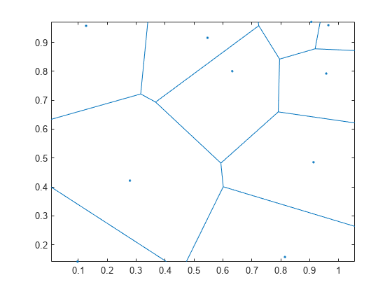
Create two vectors containing the coordinates of 10 2-D points, and plot the Voronoi diagram.
rng default;
x = rand([1 10]);
y = rand([1 10]);
voronoi(x,y)
axis equal
Input Arguments
Output Arguments
More About
Extended Capabilities
Version History
Introduced before R2006a