fsolve
Solve system of nonlinear equations
Syntax
Description
Nonlinear system solver
Solves a problem specified by
F(x) = 0
for x, where F(x) is a function that returns a vector value.
x is a vector or a matrix; see Matrix Arguments.
x = fsolve(fun,x0)x0 and tries to solve the equations fun(x) = 0,
an array of zeros.
Note
Passing Extra Parameters explains how
to pass extra parameters to the vector function fun(x),
if necessary. See Solve Parameterized Equation.
x = fsolve(fun,x0,options)options.
Use optimoptions to set these
options.
Examples
This example shows how to solve two nonlinear equations in two variables. The equations are
Convert the equations to the form .
The root2d.m function, which is available when you run this example, computes the values.
type root2d.mfunction F = root2d(x) F(1) = exp(-exp(-(x(1)+x(2)))) - x(2)*(1+x(1)^2); F(2) = x(1)*cos(x(2)) + x(2)*sin(x(1)) - 0.5;
Solve the system of equations starting at the point [0,0].
fun = @root2d; x0 = [0,0]; x = fsolve(fun,x0)
Equation solved. fsolve completed because the vector of function values is near zero as measured by the value of the function tolerance, and the problem appears regular as measured by the gradient. <stopping criteria details>
x = 1×2
0.3532 0.6061
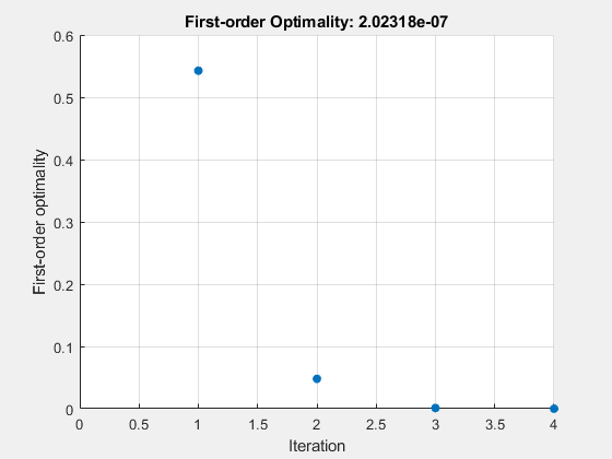
Examine the solution process for a nonlinear system.
Set options to have no display and a plot function that displays the first-order optimality, which should converge to 0 as the algorithm iterates.
options = optimoptions("fsolve",... Display="none",PlotFcn=@optimplotfirstorderopt);
The equations in the nonlinear system are
Convert the equations to the form .
The root2d function computes the left-hand side of these two equations.
function F = root2d(x) F(1) = exp(-exp(-(x(1)+x(2)))) - x(2)*(1+x(1)^2); F(2) = x(1)*cos(x(2)) + x(2)*sin(x(1)) - 0.5; end
Solve the nonlinear system starting from the point [0,0] and observe the solution process.
fun = @root2d; x0 = [0,0]; x = fsolve(fun,x0,options)
x = 1×2
0.3532 0.6061
You can parameterize equations as described in the topic Passing Extra Parameters. For example, the paramfun helper function at the end of this example creates the following equation system parameterized by :
To solve the system for a particular value, in this case , set in the workspace and create an anonymous function in x from paramfun.
c = -1; fun = @(x)paramfun(x,c);
Solve the system starting from the point x0 = [0 1].
x0 = [0 1]; x = fsolve(fun,x0)
Equation solved.

fsolve completed because the vector of function values is near zero
as measured by the value of the function tolerance, and
the problem appears regular as measured by the gradient.

<stopping criteria details>
x = 1×2
0.1976 0.4255
To solve for a different value of , enter in the workspace and create the fun function again, so it has the new value.
c = -2;
fun = @(x)paramfun(x,c); % fun now has the new c value
x = fsolve(fun,x0)Equation solved. fsolve completed because the vector of function values is near zero as measured by the value of the function tolerance, and the problem appears regular as measured by the gradient. <stopping criteria details>
x = 1×2
0.1788 0.3418
Helper Function
This code creates the paramfun helper function.
function F = paramfun(x,c) F = [ 2*x(1) + x(2) - exp(c*x(1)) -x(1) + 2*x(2) - exp(c*x(2))]; end
Create a problem structure for fsolve and solve the problem.
Solve the same problem as in Solution with Nondefault Options, but formulate the problem using a problem structure.
Set options for the problem to have no display and a plot function that displays the first-order optimality, which should converge to 0 as the algorithm iterates.
problem.options = optimoptions("fsolve",... Display="none",PlotFcn=@optimplotfirstorderopt);
The equations in the nonlinear system are
Convert the equations to the form .
The root2d function computes the left-hand side of these two equations.
function F = root2d(x) F(1) = exp(-exp(-(x(1)+x(2)))) - x(2)*(1+x(1)^2); F(2) = x(1)*cos(x(2)) + x(2)*sin(x(1)) - 0.5; end
Create the remaining fields in the problem structure.
problem.objective = @root2d;
problem.x0 = [0,0];
problem.solver = "fsolve";Solve the problem.
x = fsolve(problem)

x = 1×2

    0.3532    0.6061
This example returns the iterative display showing the solution process for the system of two equations and two unknowns
Rewrite the equations in the form :
Start your search for a solution at x0 = [-5 -5].
First, write a function that computes F, the values of the equations at x.
F = @(x) [2*x(1) - x(2) - exp(-x(1));
-x(1) + 2*x(2) - exp(-x(2))];Create the initial point x0.
x0 = [-5;-5];
Set options to return iterative display.
options = optimoptions("fsolve",Display="iter");
Solve the equations.
[x,fval] = fsolve(F,x0,options)
Norm of First-order Trust-region
Iteration Func-count ||f(x)||^2 step optimality radius
0 3 47071.2 2.29e+04 1
1 6 12003.4 1 5.75e+03 1
2 9 3147.02 1 1.47e+03 1
3 12 854.452 1 388 1
4 15 239.527 1 107 1
5 18 67.0412 1 30.8 1
6 21 16.7042 1 9.05 1
7 24 2.42788 1 2.26 1
8 27 0.032658 0.759511 0.206 2.5
9 30 7.03149e-06 0.111927 0.00294 2.5
10 33 3.29525e-13 0.00169132 6.36e-07 2.5
Equation solved.

fsolve completed because the vector of function values is near zero
as measured by the value of the function tolerance, and
the problem appears regular as measured by the gradient.

<stopping criteria details>
x = 2×1

    0.5671
    0.5671
fval = 2×1
10-6 ×

   -0.4059
   -0.4059
The iterative display shows f(x), which is the square of the norm of the function F(x). This value decreases to near zero as the iterations proceed. The first-order optimality measure likewise decreases to near zero as the iterations proceed. These entries show the convergence of the iterations to a solution. For the meanings of the other entries, see Iterative Display.
The fval output gives the function value F(x), which should be zero at a solution (to within the FunctionTolerance tolerance).
Find a matrix that satisfies
,
starting at the point x0 = [1,1;1,1]. Create an anonymous function that calculates the matrix equation and create the point x0.
fun = @(x)x*x*x - [1,2;3,4];
x0 = ones(2);
Set options to have no display.
options = optimoptions("fsolve",Display="off");
Examine the fsolve outputs to see the solution quality and process.
[x,fval,exitflag,output] = fsolve(fun,x0,options)
x = 2×2

   -0.1291    0.8602
    1.2903    1.1612
fval = 2×2
10-9 ×

   -0.2740    0.1257
    0.1884   -0.0858
exitflag =
1
output = struct with fields:
       iterations: 11
        funcCount: 52
        algorithm: 'trust-region-dogleg'
    firstorderopt: 4.0012e-10
          message: 'Equation solved.↵↵fsolve completed because the vector of function values is near zero↵as measured by the value of the function tolerance, and↵the problem appears regular as measured by the gradient.↵↵<stopping criteria details>↵↵Equation solved. The sum of squared function values, r = 1.337650e-19, is less than↵sqrt(options.FunctionTolerance) = 1.000000e-03. The relative norm of the gradient of r,↵4.001213e-10, is less than options.OptimalityTolerance = 1.000000e-06.'
The exit flag value 1 indicates that the solution is reliable. To verify this manually, calculate the residual (sum of squares of fval) to see how close it is to zero.
sum(sum(fval.*fval))
ans =
1.3376e-19
This small residual confirms that x is a solution.
You can see in the output structure how many iterations and function evaluations fsolve performed to find the solution.
Input Arguments
Output Arguments
Limitations
The function to be solved must be continuous.
When successful,
fsolveonly gives one root.The default trust-region dogleg method can only be used when the system of equations is square, i.e., the number of equations equals the number of unknowns. For the Levenberg-Marquardt method, the system of equations need not be square.
More About

Tips
For large problems, meaning those with thousands of variables or more, save memory (and possibly save time) by setting the
Algorithmoption to'trust-region'and theSubproblemAlgorithmoption to'cg'.
Algorithms
The Levenberg-Marquardt and trust-region methods are based on
the nonlinear least-squares algorithms also used in lsqnonlin. Use one of these methods if
the system may not have a zero. The algorithm still returns a point
where the residual is small. However, if the Jacobian of the system
is singular, the algorithm might converge to a point that is not a
solution of the system of equations (see Limitations).
By default
fsolvechooses the trust-region dogleg algorithm. The algorithm is a variant of the Powell dogleg method described in [8]. It is similar in nature to the algorithm implemented in [7]. See Trust-Region-Dogleg Algorithm.The trust-region algorithm is a subspace trust-region method and is based on the interior-reflective Newton method described in [1] and [2]. Each iteration involves the approximate solution of a large linear system using the method of preconditioned conjugate gradients (PCG). See Trust-Region Algorithm.
The Levenberg-Marquardt method is described in references [4], [5], and [6]. See Levenberg-Marquardt Method.
Alternative Functionality
App
The Optimize Live Editor task provides a visual interface for fsolve.
References
[1] Coleman, T.F. and Y. Li, “An Interior, Trust Region Approach for Nonlinear Minimization Subject to Bounds,” SIAM Journal on Optimization, Vol. 6, pp. 418-445, 1996.
[2] Coleman, T.F. and Y. Li, “On the Convergence of Reflective Newton Methods for Large-Scale Nonlinear Minimization Subject to Bounds,” Mathematical Programming, Vol. 67, Number 2, pp. 189-224, 1994.
[3] Dennis, J. E. Jr., “Nonlinear Least-Squares,” State of the Art in Numerical Analysis, ed. D. Jacobs, Academic Press, pp. 269-312.
[4] Levenberg, K., “A Method for the Solution of Certain Problems in Least-Squares,” Quarterly Applied Mathematics 2, pp. 164-168, 1944.
[5] Marquardt, D., “An Algorithm for Least-squares Estimation of Nonlinear Parameters,” SIAM Journal Applied Mathematics, Vol. 11, pp. 431-441, 1963.
[6] Moré, J. J., “The Levenberg-Marquardt Algorithm: Implementation and Theory,” Numerical Analysis, ed. G. A. Watson, Lecture Notes in Mathematics 630, Springer Verlag, pp. 105-116, 1977.
[7] Moré, J. J., B. S. Garbow, and K. E. Hillstrom, User Guide for MINPACK 1, Argonne National Laboratory, Rept. ANL-80-74, 1980.
[8] Powell, M. J. D., “A Fortran Subroutine for Solving Systems of Nonlinear Algebraic Equations,” Numerical Methods for Nonlinear Algebraic Equations, P. Rabinowitz, ed., Ch.7, 1970.
Extended Capabilities
Version History
Introduced before R2006aSee Also
fzero | lsqcurvefit | lsqnonlin | optimoptions | Optimize