extractHOGFeatures
Extract histogram of oriented gradients (HOG) features
Syntax
Description
features = extractHOGFeatures(I)I.
The features are returned in a 1-by-N vector, where N is
the HOG feature length. The returned features encode local shape information
from regions within an image. You can use this information for many
tasks including classification, detection, and tracking.
[ returns
HOG features extracted around specified point locations. The function
also returns features,validPoints]
= extractHOGFeatures(I,points)validPoints, which contains the
input point locations whose surrounding region is fully contained
within I. Scale information associated with the
points is ignored.
[___, optionally
returns a HOG feature visualization. You can display this visualization using
visualization]
= extractHOGFeatures(I,points)plot(visualization).
[___] = extractHOGFeatures(___, uses
additional options specified by one or more Name,Value pair arguments,
using any of the preceding syntaxes.Name,Value)
Examples
Read the image of interest.
img = imread('cameraman.tif');Extract HOG features.
[featureVector,hogVisualization] = extractHOGFeatures(img);
Plot HOG features over the original image.
figure;
imshow(img);
hold on;
plot(hogVisualization);
Read the image of interest.
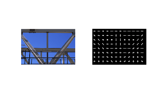
I1 = imread('gantrycrane.png');Extract HOG features.
[hog1,visualization] = extractHOGFeatures(I1,'CellSize',[32 32]);Display the original image and the HOG features.
subplot(1,2,1);
imshow(I1);
subplot(1,2,2);
plot(visualization);
Read in the image of interest.
I2 = imread('gantrycrane.png');Detect and select the strongest corners in the image.
corners   = detectFASTFeatures(im2gray(I2));
strongest = selectStrongest(corners,3);
Extract HOG features.
[hog2,validPoints,ptVis] = extractHOGFeatures(I2,strongest);
Display the original image with an overlay of HOG features around the strongest corners.
figure;
imshow(I2);
hold on;
plot(ptVis,'Color','green');

Input Arguments
Name-Value Arguments
Output Arguments
Extracted HOG features, returned as either a 1-by-N vector or a P-by-Q matrix. The features encode local shape information from regions or from point locations within an image. You can use this information for many tasks including classification, detection, and tracking.
features output | Description |
|---|---|
| 1-by-N vector | HOG feature length, N, is based on the image
size and the function parameter values. N = prod([BlocksPerImage, BlockSize, NumBins])BlocksPerImage = floor((size(I)./CellSize – BlockSize)./(BlockSize – BlockOverlap)
+ 1) |
| P-by-Q matrix | P is the number of valid points whose surrounding
region is fully contained within the input image. You provide the points input
value for extracting point locations.The surrounding region is calculated as: CellSize.*BlockSize. The feature vector length, Q, is calculated as: prod([NumBins,BlockSize]). |
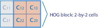
The figure below shows an image with six cells.
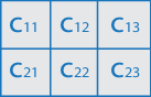
If you set the BlockSize to [2
2], it would make the size of each HOG block, 2-by-2 cells.
The size of the cells are in pixels. You can set it with the CellSize property.
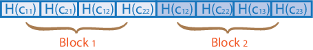
The HOG feature vector
is arranged by HOG blocks. The cell histogram, H(Cyx),
is 1-by-NumBins.
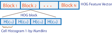
The figure below shows the HOG feature vector with a 1-by-1 cell overlap between blocks.
Valid points associated with each features descriptor vector output. This
output can be returned as either a cornerPoints object, BRISKPoints, SURFPoints object, MSERRegions object, ORBPoints object or an M-by-2 matrix of
[x,y] coordinates. The function
extracts M number of descriptors from valid interest
points in a region of size equal to
[CellSize.*BlockSize]. The
extracted descriptors are returned as the same type of object or matrix as
the input. The region must be fully contained within the image.
HOG feature visualization, returned as an object. The function
outputs this optional argument to visualize the extracted HOG features.
You can use the plot method with the visualization output.
See the Extract and Plot HOG Features example.
HOG features are visualized using a grid of uniformly spaced rose plots. The cell size and the size
of the image determines the grid dimensions. Each rose plot shows
the distribution of gradient orientations within a HOG cell. The length
of each petal of the rose plot is scaled to indicate the contribution
each orientation makes within the cell histogram. The plot displays
the edge directions, which are normal to the gradient directions.
Viewing the plot with the edge directions allows you to better understand
the shape and contours encoded by HOG. Each rose plot displays two
times NumBins petals.
You can use the following syntax to plot the HOG features:
plot(visualization) plots the HOG features
as an array of rose plots. |
plot(visualization,AX) plots HOG features
into the axes AX. |
plot(___,'Color',colorValue) Specifies the color used to plot HOG
features, where colorValue represents the color
as a 1-by-3 RGB vector, a short, or a long color name, described in
the Color
Value table. |
More About
| Color Name | Short Name | RGB Triplet | Appearance |
|---|---|---|---|
"red" | "r" | [1 0 0] |
|
"green" | "g" | [0 1 0] |
|
"blue" | "b" | [0 0 1] |
|
"cyan"
| "c" | [0 1 1] |
|
"magenta" | "m" | [1 0 1] |
|
"yellow" | "y" | [1 1 0] |
|
"black" | "k" | [0 0 0] |
|
"white" | "w" | [1 1 1] |
|
References
[1] Dalal, N. and B. Triggs. "Histograms of Oriented Gradients for Human Detection", IEEE Computer Society Conference on Computer Vision and Pattern Recognition, Vol. 1 (June 2005), pp. 886–893.
Extended Capabilities
Version History
Introduced in R2013b