Real Options Valuation with MATLAB: A Mining Economics Case Study
By David Willingham, MathWorks
Committing to the development of a major business initiative, such as a new mine, involves vast amounts of capital expenditure and long time frames—in some cases, up to 30 years. In order to understand the mine’s future economic potential and all associated risks, an accurate risk/return forecast is essential. Traditional spreadsheet solutions, which may use average values or simplistic distributions, often result in inaccurate forecasts that do not adequately assess all possible economic upside and downside risks. A more reliable approach is to use real options valuation.
In real options valuation, a separate model is created for each aspect of the project. The models are then used to simulate distributions of outcomes for different economic scenarios. Using the resultant scenarios, analysts can more accurately assess the upside and downside economic risks and recommend possible responses, such as deferring, abandoning, expanding, staging, or contracting capital investment in the project.
This article shows how MATLAB® can be used to develop and formalize a process for real options valuation of an iron ore mine. Topics include developing price and interest-rate models based on historical data and producing distributions for a range of possible economic outcomes based on calculations of net present value (NPV).

Using Net Present Value to Determine Future Profit
NPV is a standard method for appraising long-term projects by determining the time value of money. It measures the present value of money today based on the present value in the future, incorporating cash inflow and outflow and taking inflation into account.
Table 1 shows sample input data for calculating a single NPV for a mine's first year of operation. The NPV is calculated based on average values for the many areas of a mine’s operation that involve uncertainty, such as iron ore prices, production rate, and costs, but it does not take into account upside and downside risks. We will need to develop models for some or all these risks. We will use these models to perform thousands of Monte Carlo simulations and generate a distribution of possible outcomes of the mine’s NPV that we can use to measure risk.
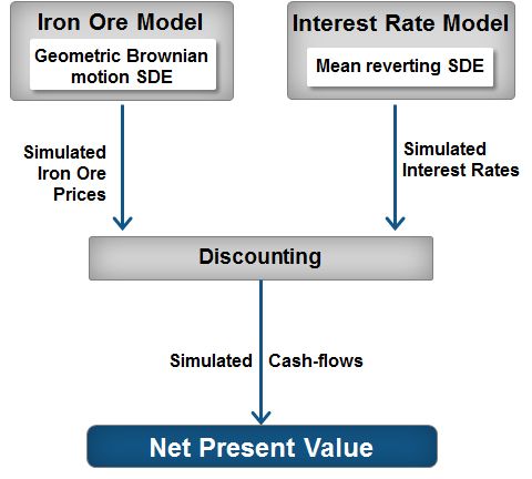
To demonstrate this approach, we will develop models for iron ore prices and interest rates (Figure 2).

Developing Iron Ore Price Models
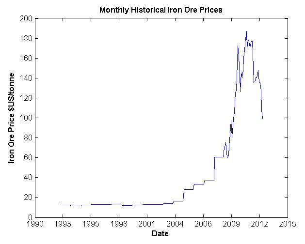
To determine what type of model we need, we review the historical iron ore prices (Figure 3). The data shows that the price of iron ore has risen sharply since 2005 and has been quite volatile for the past five years. Speculators believe that the rise is due to the strong growth in China and India, and that it will remain high until economic growth in those countries starts to slow.
We will simulate two models: a returns-based model based on the assumption that the price will continue to fluctuate for the next two years, and a mean-reversion model based on the assumption that the price will remain stable over that period.
We will use stochastic differential equations (SDEs) to create both models. (SDEs are a typical approach to modeling and simulating uncertain phenomena, such as fluctuating stock prices.)
For the returns-based model, we create a geometric Brownian motion (GBM) SDE. It can be described as:
\[dX_t=\mu*X_t*dt+\sigma*X_t*dW_t\]
where
\(\mu = \) Instantaneous rate of return
\(\sigma =\) Volatility rate
For the mean reversion model, we use a Hull-White/Vasicek SDE with mean-reverting drift:
\[dX_t=\alpha*(\mu- X_t)*dt+\sigma*dW_t\]
where
\(\alpha =\) Mean reversion rate
\(\mu =\) Mean level
\(\sigma =\) Volatility
Using the gbm and hwv functions in Econometrics Toolbox™, we can create both models in a few lines of code.
Using gbm, the code is as follows:
     sigma = std(returns);
     mu = mean(returns);
     model = gbm(mu,sigma,'StartState', startdate);
Using hwv, the code is:
     regressors = [ones(length(returns) - 1, 1) returns(1:end-1)];
     [coefficients, intervals, residuals] = regress(diff(returns), regressors);
     dt    = 1;
     speed = -coefficients(2)/dt;
     level = -coefficients(1)/coefficients(2);
     sigma =  std(residuals)/sqrt(dt);
     model = hwv(speed,level,sigma,  'StartState',startdate);
Once we have created the models, we simulate them using the forecasted time frame, number of simulations, and type of model as inputs:
     NTrials = 1000;
     years = 8;
     ann = 12;
     NSteps = years*ann;
     tic
     Xsim = simulate(model, NSteps, 'NTrials', NTrials, 'DeltaTime', dt);
     Xsim = squeeze(Xsim); % Remove redundant dimension
     toc
     Elapsed time is 0.026889 seconds.
Note that it took only a fraction of a second to complete 1000 simulations.
Figures 4 and 5 show the simulation results for each model.
Each model predicts a different outcome in response to a downturn in prices: With the GBM model the forecasts trend downwards, while with the HWV model, they return to a mean. With these two models available, we will be able to plan for both scenarios.
Modeling Interest Rates
Interest rates tend to revert to a mean; in Australia, that has been the case for the past 30 years. For this reason, we will use the HWV model, modifying it to reflect historical interest rates.
Figure 6 shows the historical interest rates, with an average mean level of 5.5%.
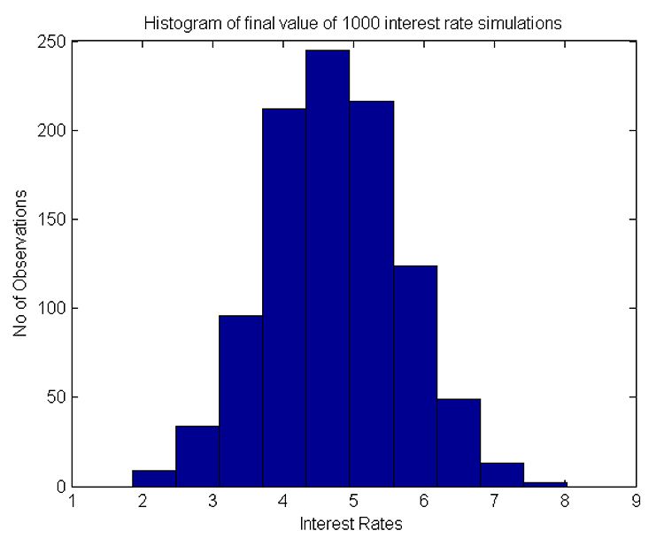
Figure 7 shows a histogram of the spread of 1000 simulations of the interest rate model with a mean of approximately 5.5%. The mean is what we expected; however, there is some upside and downside risk with the tails of the interest rates +/- 2.5% (or 50% away from the mean).
Calculating Net Present Value
The final task is to calculate the discounted cash flow and the final NPV of the mine.
NPV can be summarized as follows:
Cashflow = Sales*Production*IronOreGrade*IronPrice
DiscountFactor = exp(-interest*timeperiod)
NPV = (Cashflow – Costs)*DiscountFactor
Now that we have calculated the NPV of the mine based on the GBM and HWV models, we can run scenarios on iron ore prices (either mean reverting or based on returns and interest rates).
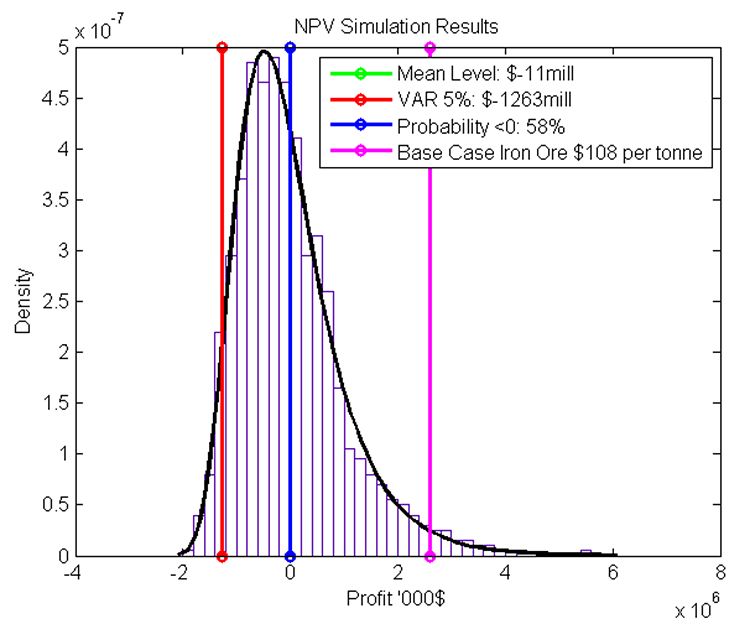
First, let’s look at a scenario that uses the HWV iron ore price model. Figure 8 shows the NPV distribution of cash flow when running this model. It also shows the cash flow values around certain outcomes, such as mean, 5% value at risk, and a base rate of $108 per tonne. Using the Distribution Fitting app in Statistics and Machine Learning Toolbox™, we calculate these values from a normal distribution for HWV and a generalized extreme value distribution for GBM. Note that in this scenario, all possible outcomes are positive, so that if iron ore prices revert to the mean, the mine should continue to be profitable.
Now let’s look at a scenario where we use the GBM model. As Figure 9 shows, some of the cash flow results are negative, and 55% of the simulations result in a negative value. If iron ore prices continue to decline, the mine should cease production until they rise again or until costs can be reduced.
Assumptions and Future Improvements
The models in our examples were chosen based on the assumption that Brownian motions of the prices and interest rates are independent and uncorrelated, whereas in reality they could be linked. To provide a more realistic forecast for NPV, the models could be jointly calibrated and simulated to introduce a correlation. The SDE framework within Econometrics Toolbox supports this level of modeling.
Reusable Forecasting
The purpose of performing real options valuation was to help us decide whether the mine should continue to operate or be put on hold. Focusing on iron ore prices and interest rates, we modeled and forecast 1000 potential outcomes of NPV using an approach that was fast, efficient, and reusable. The two scenarios produced very different outcomes, resulting in different “real options.” We would need to compare each model with actual prices and then rerun the models to see whether the outcomes change with time.
Published 2013 - 92117v00


