Simulating Blackjack with MATLAB
By Cleve Moler, MathWorks
Blackjack is the most popular casino game in the world. Using a basic strategy, a knowledgeable player can reduce the casino's advantage to less than one-half of one percent. Simulating blackjack play with this strategy in MATLAB® is both an instructive programming exercise and a useful parallel computing benchmark.
Blackjack is also known as "21." The object is to get a hand with a value close to, but not more than, 21. Face cards are worth 10 points, aces are worth either 1 or 11, and all other cards are worth their numerical value. You play against the dealer. You each start with two cards. Your cards are dealt face up; one of the dealer's cards stays face down.
You signal "hit" to receive additional cards. When you are satisfied with your hand, you "stand." The dealer then reveals the hidden card and finishes the hand. If your total ever exceeds 21, you are "bust," and the dealer wins the hand without drawing any more cards.
The dealer has no choices to make, and must draw on hands worth less than 17 and stand on hands worth 17 or more. (A variant has the dealer draw to a "soft" 17, which is a hand with an ace counting 11.) If neither player goes bust, then the hand closest to 21 wins. Equal totals are a "push," and neither wins.
The fact that you can bust before the dealer takes any cards is a disadvantage that would be overwhelming were it not for three additional features of the game. On your first two cards:
- An ace and a face card or a 10 is a "blackjack," which pays 1.5 times the bet if the dealer does not also have 21
- You can "split" a pair into two separate hands by doubling the bet
- You can "double down" a good hand by doubling the bet and receiving just one more card
Basic Strategy
Basic strategy was first described in the 1956 paper "The Optimum Strategy in Blackjack," published in the Journal of the American Statistical Association by four authors from the Aberdeen Proving Ground. It is now presented, with a few variations, on dozens of web pages, including Wikipedia. The strategy assumes that you do not retain information from earlier hands. Your play depends only on your current hand and the dealer's up card. With basic strategy, the house advantage is only about one half of one percent of the original bet.
My MATLAB programs, shown in the sidebar, use three functions to implement basic strategy. The function hard uses the array HARD to guide the play of most hands. The row index into HARD is the current total score, and the column index is the value of the dealer's up card. The return value is 0, 1, or 2, indicating "stand," "hit," or "double down." The other two functions, soft and pair, play similar roles for hands containing an ace worth 11 and hands containing a pair.
The most important consideration in basic strategy is to avoid going bust when the dealer has a chance of going bust. In our functions, the subarray HARD(12:16,2:6) is nearly all zero. This represents the situation where both you and the dealer have bad hands—your total and the dealer's expected total are each less than 17. You are tempted to hit, but you might bust, so you stand. The dealer will have to hit, and might bust. This is your best defense against the house advantage. With naïve play, which ignores the dealer's up card, you would almost certainly hit a 12 or 13. But if the dealer is also showing a low card, stand on your low total and wait to see if the dealer goes over 21.
Card Counting
Card counting was introduced in 1962 in Beat the Dealer, a hugely popular book by Edward Thorp. If the deck is not reshuffled after every hand, you can keep track of, for example, the number of aces, face cards, and nonface cards that you have seen. As you approach the end of the deck, you may know that it is “ten rich”—the number of aces and face cards remaining is higher than would be expected in a freshly shuffled deck. This situation is to your advantage because you have a better than usual chance of getting a blackjack and the dealer has a better than usual chance of going bust. So you increase your bet and adjust your strategy.
Card counting gives you a mathematical advantage over the casino. Exactly how much of an advantage depends upon how much you are able to remember about the cards you have seen. Thorp's book was followed by a number of other books that simplified and popularized various systems. My personal interest in blackjack began with a 1973 book by John Archer. But I can attest that card counting is boring, error-prone, and not very lucrative. It is nowhere near as glamorous—or as dangerous—as the recent Hollywood film "21" portrays it. And many venues now have machines that continuously shuffle the cards after each hand, making card counting impossible.
The MATLAB Simulations
My original MATLAB program, written several years ago, had a persistent array that is initialized with a random permutation of several copies of the vector 1:52. These integers represent both the values and the suits in a 52-card deck. The suit is irrelevant in the play, but is nice to have in the display. Cards are dealt from the end of the deck, and the deck is reshuffled when there are just a few cards left.
function card = dealcard
% Deal one card
persistent deck
if length(deck) < 10
   % Four decks
   deck = [1:52 1:52 1:52 1:52];
   % Shuffle
   deck = deck(randperm(length(deck)));
end
card = deck(end);
deck(end) = [];
This function faithfully simulates a blackjack game with four decks dealt without reshuffling between hands. It would be possible to count cards, but this shuffler has two defects: It does not simulate a modern shuffling machine, and the persistent array prevents some kinds of parallelization.
My most recent simulated shuffler is much simpler. It creates an idealized mechanical shuffler that has an infinite number of perfectly mixed decks. It is not possible to count cards with this shuffler.
function card = dealcard
% Deal one card
card = ceil(52*rand);
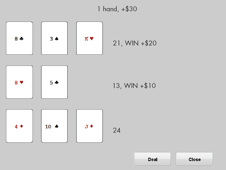
I have two blackjack programs, both available on MATLAB Central. One program offers an interface that lets you play one hand at a time. Basic strategy is highlighted, but you can make other choices. For example, Figures 1 and 2 show the play of an infrequent but lucrative hand. You bet $10 and are dealt a pair of 8s. The dealer's up card is a 4. Basic strategy recommends splitting the pair of 8s. This increases the bet to $20. The first hand is then dealt a 3 to add to the 8, giving 11. Basic strategy recommends always doubling down on 11. This increases the total bet to $30. The next card is a king, giving the first hand 21. The second hand is dealt a 5 to go with the 8, giving it 13. You might be tempted to hit the 13, but the dealer is showing a 4, so you stand. The dealer reveals a 10, and has to hit the 14. The final card is a jack, busting the dealer and giving you $30. This kind of hand is rare, but gratifying to play correctly.
My second program plays a large number of hands using basic strategy and collects statistics about the outcome.
Accelerating the Simulations with Parallel Computing
I like to demonstrate parallel computing with MATLAB by running several copies of my blackjack simulator simultaneously using Parallel Computing Toolbox™. Here is the main program:
% BLACKJACKDEMO Parallel blackjack demo.
matlabpool
p = 4;      % Number of players.
n = 25000;  % Number of hands per player.
B = zeros(n,p);
parfor k = 1:p
   B(:,k) = blackjacksim(n);
end
plot(cumsum(B))
r = sum(B(n,1:p));
fmt = '%d x %d hands, total return = $ %d'
title(sprintf(fmt,p,n,r))
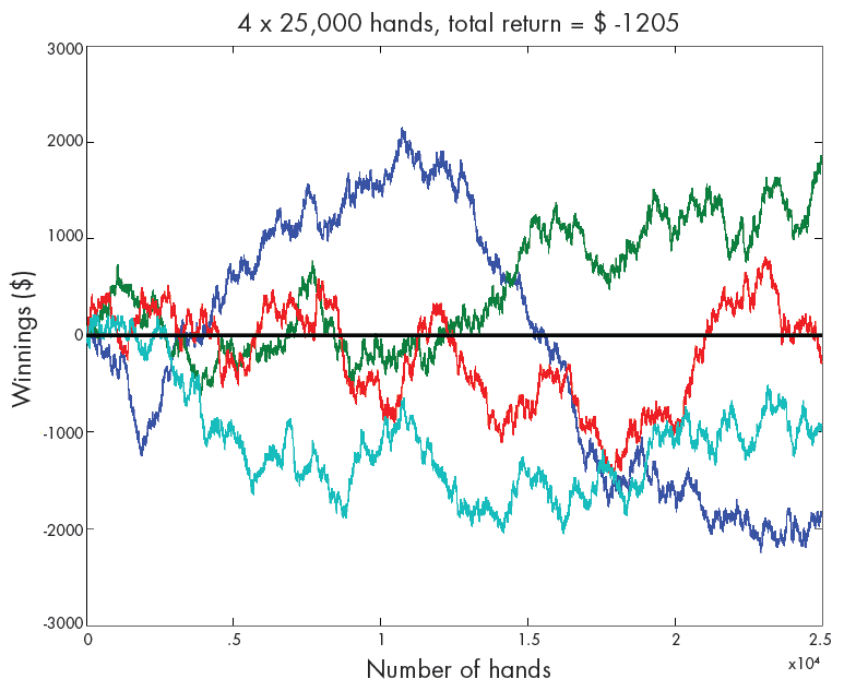
The matlabpool command starts up many workers (copies of MATLAB) on the cores or processors available in a multicore machine or a cluster. These workers are also known as labs. The random number generators on each lab are initialized to produce statistically independent streams drawn from a single overall global stream. The main program on the master MATLAB creates an array B, and then the parfor loop runs a separate instance of the sequential simulator, blackjacksim, on each lab. The results are communicated to the master and stored in the columns of B. The master can then use B to produce the plot shown in Figure 3. With "only" 25,000 hands for each player, the simulation is still too short to show the long-term trend. The computation time is about 11 seconds on my dual-core laptop. If I do not turn on the MATLAB pool, the computation uses only one core and takes almost 20 seconds.
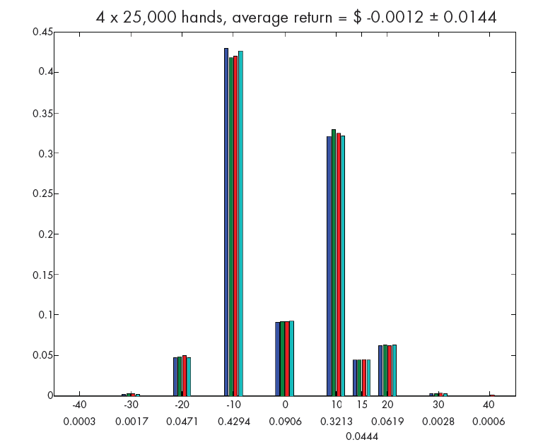
This run can also produce the histograms shown in Figure 4. The cumulative return from the four players is the dot product of the two vectors annotating the horizontal axis. The discrepancy between the frequency of $10 wins and $10 losses is almost completely offset by the higher frequencies of the larger wins over the larger losses. The average return and a measure of its variation are shown in the title of the figure. We see that in runs of this length, the randomness of the shuffle still dominates. It would require longer runs with millions of hands to be sure that the expected return is slightly negative.
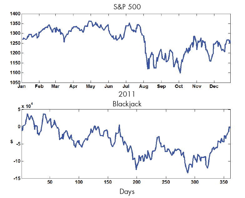
Blackjack can be a surrogate for more sophisticated financial instruments. The first graph in Figure 5 shows the performance of the Standard & Poor's stock market index during 2011. The second shows the performance of our blackjack simulation playing 100 hands a day for each of the 252 days the stock market was open that year. The S&P dropped 14.27 points. Our blackjack simulation, which bet $10 per hand, lost $3860 over the same period. More important than these final results is the fact that both instruments show large fluctuations about their mean behavior. Over the short term, stock market daily behavior and card shuffling luck are more influential than any long-term trend.
MATLAB Functions for Basic Blackjack Strategy
function strat = hard(p,d)
   % Hands without aces.
   % hard(player,dealer)
   % 0 = stand
   % 1 = hit
   % 2 = double down
   % Dealer shows:
   %      2 3 4 5 6 7 8 9 T A
   HARD = [ ...
      1   x x x x x x x x x x
      2   1 1 1 1 1 1 1 1 1 1
      3   1 1 1 1 1 1 1 1 1 1
      4   1 1 1 1 1 1 1 1 1 1
      5   1 1 1 1 1 1 1 1 1 1
      6   1 1 1 1 1 1 1 1 1 1
      7   1 1 1 1 1 1 1 1 1 1
      8   1 1 1 1 1 1 1 1 1 1
      9   2 2 2 2 2 1 1 1 1 1
     10   2 2 2 2 2 2 2 2 1 1
     11   2 2 2 2 2 2 2 2 2 2
     12   1 1 0 0 0 1 1 1 1 1
     13   0 0 0 0 0 1 1 1 1 1
     14   0 0 0 0 0 1 1 1 1 1
     15   0 0 0 0 0 1 1 1 1 1
     16   0 0 0 0 0 1 1 1 1 1
     17   0 0 0 0 0 0 0 0 0 0
     18   0 0 0 0 0 0 0 0 0 0
     19   0 0 0 0 0 0 0 0 0 0
     20   0 0 0 0 0 0 0 0 0 0];
   strat = HARD(p,d);
end

function strat = soft(p,d)
   % Hands with aces.
   % soft(player-11,dealer)
   % 0 = stand
   % 1 = hit
   % 2 = double down
   % Dealer shows:
   %      2 3 4 5 6 7 8 9 T A
   SOFT = [ ...
      1   1 1 1 1 1 1 1 1 1 1
      2   1 1 2 2 2 1 1 1 1 1
      3   1 1 2 2 2 1 1 1 1 1
      4   1 1 2 2 2 1 1 1 1 1
      5   1 1 2 2 2 1 1 1 1 1
      6   2 2 2 2 2 1 1 1 1 1
      7   0 2 2 2 2 0 0 1 1 0
      8   0 0 0 0 0 0 0 0 0 0
      9   0 0 0 0 0 0 0 0 0 0];
   strat = SOFT(p,d);
end

function strat = pair(p,d)
   % Strategy for splitting pairs.
   % pair(paired,dealer)
   % 0 = keep pair
   % 1 = split pair
   % Dealer shows:
   %      2 3 4 5 6 7 8 9 T A
   PAIR = [ ...
      1   x x x x x x x x x x
      2   1 1 1 1 1 1 0 0 0 0
      3   1 1 1 1 1 1 0 0 0 0
      4   0 0 0 1 0 0 0 0 0 0
      5   0 0 0 0 0 0 0 0 0 0
      6   1 1 1 1 1 1 0 0 0 0
      7   1 1 1 1 1 1 1 0 0 0
      8   1 1 1 1 1 1 1 1 1 1
      9   1 1 1 1 1 0 1 1 0 0
     10   0 0 0 0 0 0 0 0 0 0
     11   1 1 1 1 1 1 1 1 1 1];
   strat = PAIR(p,d);
end
x = NaN; % Not possible
Published 2012 - 92052v00
References
-
Baldwin, R. R., Cantey, W. E., Maisel, H., and McDermot, J. P. “The Optimum Strategy in Blackjack,” Journal of the American Statistical Association, 51:429-439 (Sept.), 1956.
-
Thorp, E. O. Beat the Dealer. New York: Random House, 1962.
-
Wikipedia. https://en.wikipedia.org/wiki/Blackjack


