raytrace
Display or compute RF propagation rays
Description
The raytrace function plots or computes propagation
paths by performing ray tracing analysis with the 3-D model defined by the Map argument. The function color-codes each propagation path according
to the received power (dBm) or path loss (dB) from the transmitter site to the receiver
site.
The ray tracing analysis includes surface reflections and edge diffractions, but does
not include effects from corner diffraction, refraction, or diffuse scattering. This
function supports frequencies from 100 MHz to 100 GHz. The function evaluates the
propagation paths for the frequencies associated with the tx input. Specify
the operating frequency of a transmitter site by using the
TransmitterFrequency property of the txsite
object. For more information about ray tracing analysis, see Ray Tracing for Wireless Communications.
raytrace(
displays the propagation paths from the transmitter site tx,rx)tx to
the receiver site rx in the current Site Viewer. By default,
the function uses the shooting and bouncing rays (SBR) method, finds paths with up
to two reflections and zero diffractions, and discards paths that are more than 40
dB weaker than the strongest path.
raytrace(
finds propagation paths using the ray tracing propagation model
tx,rx,propmodel)propmodel. Ray tracing propagation models enable you to
specify properties such as the maximum number of reflections and diffractions, path
loss thresholds, and building and terrain materials. Create a ray tracing
propagation model by using the propagationModel function.
raytrace(___,
specifies options using one or more name-value arguments, in addition to any
combination of inputs from the previous syntaxes.Name=Value)
rays = raytrace(___)rays.
Examples
Show reflected propagation paths in Chicago using a ray tracing propagation model.
Launch Site Viewer with buildings in Chicago. For more information about the OpenStreetMap® file, see [1].
viewer = siteviewer(Buildings="chicago.osm");Create a transmitter site and a receiver site near two different buildings.
tx = txsite(Latitude=41.8800, ...
    Longitude=-87.6295, ...
    TransmitterFrequency=2.5e9);
show(tx)
rx = rxsite(Latitude=41.8813452, ...
    Longitude=-87.629771, ...
    AntennaHeight=30);
show(rx)
Show the obstruction to the line-of-sight path.
los(tx,rx)
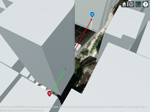
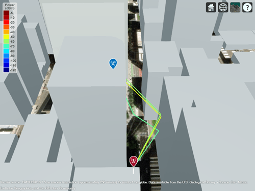
Display propagation paths with reflections. By default, the raytrace function uses the SBR method and calculates propagation paths with up to two reflections.
raytrace(tx,rx)
Appendix
[1] The OpenStreetMap file is downloaded from https://www.openstreetmap.org, which provides access to crowd-sourced map data all over the world. The data is licensed under the Open Data Commons Open Database License (ODbL), https://opendatacommons.org/licenses/odbl/.
Launch Site Viewer with buildings in Chicago. For more information about the OpenStreetMap® file, see [1].
viewer = siteviewer(Buildings="chicago.osm");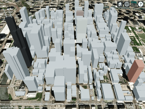
Create a transmitter site on a building.
tx = txsite(Latitude=41.8800, ...
    Longitude=-87.6295, ...
    TransmitterFrequency=2.5e9);
Create a receiver site near another building.
rx = rxsite(Latitude=41.881352, ...
    Longitude=-87.629771, ...
    AntennaHeight=30);
Create a ray tracing propagation model, which MATLAB® represents using a RayTracing object. By default, the propagation model uses the SBR method and finds propagation paths with up to two surface reflections.
pm = propagationModel("raytracing");Calculate the signal strength using the receiver site, the transmitter site, and the propagation model.
ssTwoReflections = sigstrength(rx,tx,pm)
ssTwoReflections =
-54.3151
Plot the propagation paths.
raytrace(tx,rx,pm)

Change the RayTracing object to find paths with up to 5 reflections. Then, recalculate the signal strength.
pm.MaxNumReflections = 5;
ssFiveReflections = sigstrength(rx,tx,pm)
ssFiveReflections =
-53.3965
By default, RayTracing objects use concrete terrain materials and building materials derived from the OpenStreetMap file. When the OpenStreetMap file does not specify materials, the model uses concrete. Change the building and terrain material types to model perfect electrical conductors.
pm.TerrainMaterial = "PEC";
pm.BuildingsMaterial = "PEC";

ssPerfect = sigstrength(rx,tx,pm)
ssPerfect =
-38.9334
Plot the propagation paths for the updated propagation model.
raytrace(tx,rx,pm)
Appendix
[1] The OpenStreetMap file is downloaded from https://www.openstreetmap.org, which provides access to crowd-sourced map data all over the world. The data is licensed under the Open Data Commons Open Database License (ODbL), https://opendatacommons.org/licenses/odbl/.
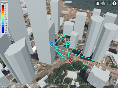
Launch Site Viewer with buildings in Hong Kong. For more information about the OpenStreetMap® file, see [1].
viewer = siteviewer(Buildings="hongkong.osm");
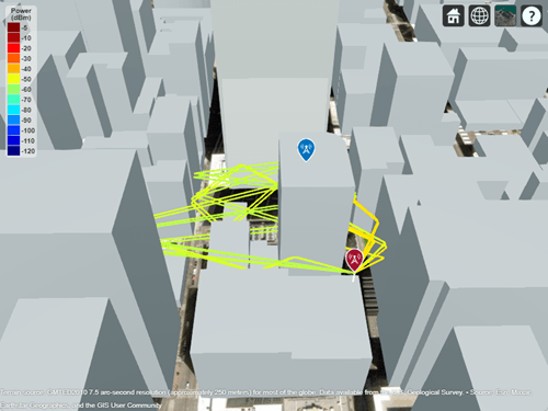
Create transmitter and receiver sites that model a small cell scenario in a dense urban environment.
tx = txsite(Name="Small cell transmitter", ...
    Latitude=22.2789, ...
    Longitude=114.1625, ...
    AntennaHeight=10, ...
    TransmitterPower=5, ...
    TransmitterFrequency=28e9);
rx = rxsite(Name="Small cell receiver", ...
    Latitude=22.2799, ...
    Longitude=114.1617, ...
    AntennaHeight=1);
Create a ray tracing propagation model, which MATLAB represents using a RayTracing object. Configure the model to use a low average number of degrees between launched rays, to find paths with up to 5 path reflections, and to use building and terrain material types that model perfect electrical conductors. By default, the model uses the SBR method.
pm = propagationModel("raytracing", ...
    MaxNumReflections=5, ...
    AngularSeparation="low", ...
    BuildingsMaterial="PEC", ...
    TerrainMaterial="PEC");
Visualize the propagation paths and calculate the corresponding path losses.
raytrace(tx,rx,pm,Type="pathloss")
raysPerfect = raytrace(tx,rx,pm,Type="pathloss");
plPerfect = [raysPerfect{1}.PathLoss]
plPerfect = 1×13

  104.2656  103.5699  112.0092  109.3137  111.2840  111.9979  112.4416  108.1505  111.2825  111.3905  117.7506  116.5906  117.7638
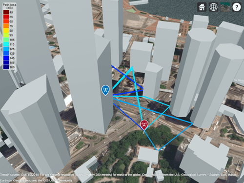
Set the building and terrain material types to glass and concrete, respectively. Then, revisualize the propagation paths and recalculate the corresponding path losses. The model finds one fewer path because, by default, the model discards paths that are more than 40 decibels weaker than the strongest path. The first path loss value does not change because it corresponds to the line-of-sight propagation path.
pm.BuildingsMaterial = "glass";
pm.TerrainMaterial = "concrete";

raytrace(tx,rx,pm,Type="pathloss")
raysMtrls = raytrace(tx,rx,pm,Type="pathloss");
plMtrls = [raysMtrls{1}.PathLoss]
plMtrls = 1×12

  104.2656  106.1249  119.2135  121.2269  122.3753  121.5228  126.8929  124.1284  122.7842  127.4910  138.9922  140.4998
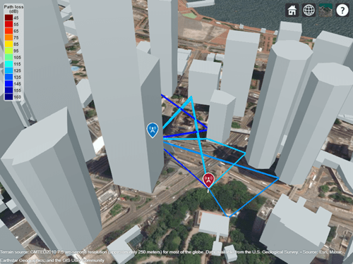
Incorporate atmospheric loss by adding rain and gas propagation models to the ray tracing model. Then, revisualize the propagation paths and recalculate the corresponding path losses.
pm = pm + propagationModel("rain") + propagationModel("gas");

raytrace(tx,rx,pm,Type="pathloss")
raysAtmospheric = raytrace(tx,rx,pm,Type="pathloss");
plAtmospheric = [raysAtmospheric{1}.PathLoss]
plAtmospheric = 1×11

  105.3233  107.1836  121.7958  123.1202  124.9592  124.1122  129.6076  126.0225  125.3745  130.2060  143.9945
Appendix
[1] The OpenStreetMap file is downloaded from https://www.openstreetmap.org, which provides access to crowd-sourced map data all over the world. The data is licensed under the Open Data Commons Open Database License (ODbL), https://opendatacommons.org/licenses/odbl/.
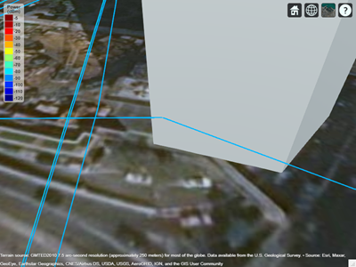
This example shows how to:
Scale an STL file so that the model uses units of meters.
View the scaled model in Site Viewer.
Use ray tracing to calculate and display propagation paths from a transmitter to a receiver.
While Cartesian txsite and rxsite objects require position coordinates in meters, STL files can use other units. If your STL file does not use meters, you must scale the model before importing it into Site Viewer.
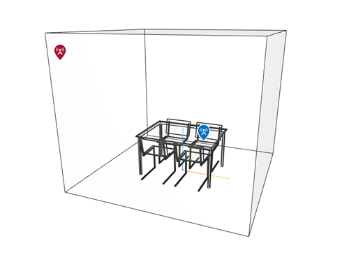
Import and view an STL file. The file models a small conference room with one table and four chairs. Scale the model by specifying the SceneModelScale name-value argument. For this example, assume that the conversion factor from the STL units to meters is 0.9.
viewer = siteviewer(SceneModel="conferenceroom.stl",SceneModelScale=0.9);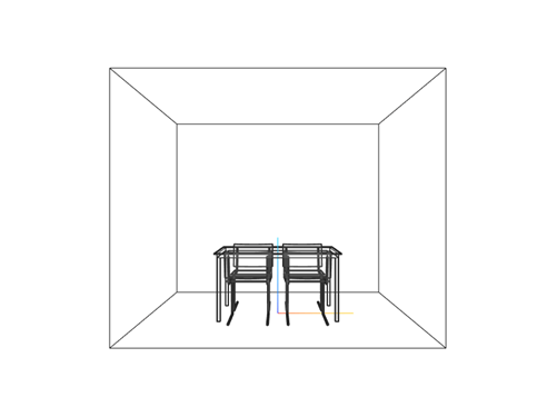
Before R2023b: Read the model into a triangulation object by using the stlread function, scale the coordinates and create a new triangulation object, and then read the new triangulation object into Site Viewer.
Create and display a transmitter site close to the wall and a receiver site under the table. Specify the position using Cartesian coordinates in meters.
tx = txsite("cartesian", ...
    AntennaPosition=[-1.25; -1.25; 1.9], ...
    TransmitterFrequency=2.8e9);
show(tx,ShowAntennaHeight=false)

rx = rxsite("cartesian", ...
    AntennaPosition=[0.3; 0.2; 0.5]);
show(rx,ShowAntennaHeight=false)
Pan by left-clicking, zoom by right-clicking or by using the scroll wheel, and rotate the visualization by clicking the middle button and dragging or by pressing Ctrl and left-clicking and dragging.
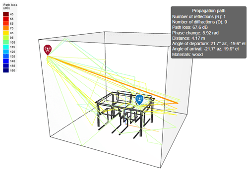
Create a ray tracing propagation model for Cartesian coordinates, which MATLAB represents using a RayTracing object. Calculate rays that have up to 1 reflection and 1 diffraction. Set the surface material to wood. By default, the model uses the SBR method.
pm = propagationModel("raytracing", ...
    CoordinateSystem="cartesian", ....
    MaxNumReflections=1, ...
    MaxNumDiffractions=1, ...
    SurfaceMaterial="wood");
Calculate the propagation paths and return the result as a cell array of comm.Ray objects. Extract and plot the rays.
r = raytrace(tx,rx,pm);
r = r{1};
plot(r)
View information about a ray by clicking on it.
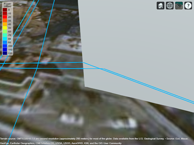
Since R2023b
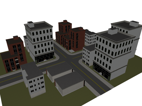
View a 3-D model from a glTF™ file created using RoadRunner. RoadRunner is an interactive editor that lets you design 3-D scenes for simulating and testing automated driving systems.
Create a temporary folder to store a sample glTF file. Download the file into the folder by using the downloadGLTFFile helper function. The helper function is attached to the example as a supporting file.
dataDir = fullfile(tempdir,"IntersectionAndBuildings");
if ~exist(dataDir,"dir")
    mkdir(dataDir)
end
downloadGLTFFile(dataDir)
Specify the name of the binary file. Then, import and view the glTF file using Site Viewer. Site Viewer displays the model using the colors and textures stored in the file.
filename = fullfile(dataDir,"IntersectionAndBuildings.glb");
viewer = siteviewer(SceneModel=filename,ShowEdges=false,ShowOrigin=false);
Adjust the view by changing the camera position and the camera rotation angles. Specify the position using meters and the rotation angles using degrees.
campos(viewer,-26,-57,37)
campitch(viewer,-25)
camheading(viewer,-26)
Site Viewer assigns materials to the surfaces in the scene by matching each material name stored in the file with the name of a supported material. View a subset of the materials and matched materials. By default, ray tracing analysis functions use the materials stored in the MatchedCatalogMaterial variable.
viewer.Materials(1:5,:)
ans=5×2 table
       Material       MatchedCatalogMaterial
    ______________    ______________________

    "Metal_Trim"            "metal"
    "Glass"                 "glass"
    "Stone_Trim"            "marble"
    "Roof_Asphalt"          "concrete"
    "Bricks_Red"            "brick"
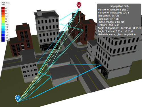
Create a transmitter site above a building and a receiver site behind a cluster of buildings. Specify the positions using Cartesian coordinates in meters.
tx = txsite("cartesian",AntennaPosition=[18;38;22]);
rx = rxsite("cartesian",AntennaPosition=[-40;-35;1]);
Create a ray tracing propagation model for Cartesian coordinates, which MATLAB® represents by using a RayTracing object. Configure the model to find propagation paths that have up to two reflections (the default) and one diffraction.
pm = propagationModel("raytracing", ...
    CoordinateSystem="cartesian", ...
    MaxNumDiffractions=1);
Calculate the propagation paths and return the result as a cell array of comm.Ray objects. Extract the propagation paths from the cell array.
rays = raytrace(tx,rx,pm);
rays = rays{1};
Display the transmitter site, the receiver site, and the propagation paths. Adjust the view by changing the camera position and the camera rotation angles.
show(tx)
show(rx)
plot(rays)

campos(viewer,-22,-78,61)
campitch(viewer,-37)
camheading(viewer,-13)
View information about a path by clicking it. The information box displays the interaction materials.
Input Arguments
Name-Value Arguments
Specify optional pairs of arguments as
Name1=Value1,...,NameN=ValueN, where Name is
the argument name and Value is the corresponding value.
Name-value arguments must appear after other arguments, but the order of the
pairs does not matter.
Example: raytrace(tx,rx,Type="pathloss") color-codes paths based
on path loss.
Before R2021a, use commas to separate each name and value, and enclose
Name in quotes.
Example: raytrace(tx,rx,"Type","pathloss") color-codes paths
based on path loss.
Type of quantity to plot, specified as one of these options:
"power"— Color-code paths based on the received power in dBm. For more information about ray tracing models calculate received power, see the Power at Receiver section of Ray Tracing for Wireless Communications."pathloss"— Color-code paths based on path loss in dB.
Data Types: char | string
Propagation model, specified as one of these options:
"raytracing"— Use the SBR method, find paths with up to two reflections and zero diffractions, and discard paths that are more than 40 dB weaker than the strongest path.RayTracingobject — Ray tracing propagation model. Create aRayTracingobject by using thepropagationModelfunction.RayTracingobjects enable you to specify properties such as the ray tracing method, the maximum number of reflections and diffractions, path loss thresholds, and building and terrain materials. For information about the differences between ray tracing methods, see Choose a Propagation Model.CompositePropagationModelobject — Composite propagation model. The model must incorporate a ray tracing propagation model. Create a composite propagation model from individual propagation models by using theaddfunction. For information about the types of propagation models that can be combined, see Choose a Propagation Model.
You can also specify the propagation model by using the
propmodel argument. If you specify both
propmodel and
PropagationModel, the function uses the value
of PropagationModel.
Data Types: char | string
Color limits for the colormap, specified as a two-element numeric row
vector of the form [min max].
The units and the default value depend on the value of
Type:
"power"– Units are in dBm, and the default value is[-120 -5]."pathloss"– Units are in dB, and the default value is[45 160].
The color limits indicate the values that map to the first and last colors in the colormap. The function does not plot propagation paths with values that are below the minimum color limit.
Data Types: double
Colormap for the propagation paths, specified as a colormap name or as an M-by-3 array of RGB triplets that define M individual colors.
This table lists the colormap names.
| Colormap Name | Color Scale |
|---|---|
|
|
|
|
|
|
|
|
|
|
|
|
|
|
|
|
|
|
|
|
|
|
|
|
|
|
|
|
|
|
|
|
|
|
|
|
|
|
|
|
|
|
|
|
Data Types: char | string | double
Show color legend in Site Viewer, specified as a numeric or logical
1 (true) or
0 (false).
Map for visualization or surface data, specified as a siteviewer
object, a triangulation object, a string scalar, or a character vector.
Valid and default values depend on the coordinate system.
| Coordinate System | Valid Map Values | Default Map Value |
|---|---|---|
"geographic" |
|
|
"cartesian" |
|
|
a Alignment of boundaries and region labels are a presentation of the feature provided by the data vendors and do not imply endorsement by MathWorks®. | ||
In most cases, if you specify this argument as a value other than a siteviewer or
"none", then you must also specify an output argument.
Output Arguments
Tips
The comm.Ray objects created by the raytrace
function calculate path loss using patterns from the antenna arrays stored in the
Antenna properties of the input txsite and rxsite objects. By
default, the raytrace function discards propagation paths that are
more than 40 dB weaker than the strongest path. As a result, when the antennas are
polarized, the raytrace function might unexpectedly discard some
comm.Ray objects. You can investigate additional propagation paths
by setting the Antenna property of the txsite and
rxsite objects to "isotropic". Alternatively,
you can create a RayTracing
propagation model object, set the MaxRelativePathLoss property of
the RayTracing object to Inf, and specify the
RayTracing object as input to the raytrace
function.
References
[1] International Telecommunications Union Radiocommunication Sector. Effects of Building Materials and Structures on Radiowave Propagation Above About 100MHz. Recommendation P.2040. ITU-R, approved August 23, 2023. https://www.itu.int/rec/R-REC-P.2040/en.
[2] International Telecommunications Union Radiocommunication Sector. Electrical Characteristics of the Surface of the Earth. Recommendation P.527. ITU-R, approved September 27, 2021. https://www.itu.int/rec/R-REC-P.527/en.
[3] Mohr, Peter J., Eite Tiesinga, David B. Newell, and Barry N. Taylor. “Codata Internationally Recommended 2022 Values of the Fundamental Physical Constants.” NIST, May 8, 2024. https://www.nist.gov/publications/codata-internationally-recommended-2022-values-fundamental-physical-constants.
[4] "IEEE Standard Definitions of Terms for Antennas." IEEE Std 145-2013 (Revision of IEEE Std 145-1993), March 2014, 1–50. https://doi.org/10.1109/IEEESTD.2014.6758443.
Extended Capabilities
Version History
Introduced in R2019bWhen you find propagation paths using the SBR method, MATLAB corrects the results so that the geometric accuracy of each path is exact, using single-precision floating-point computations. In previous releases, the paths have approximate geometric accuracy.
For example, this code finds propagation paths between a transmitter and receiver
by using the default SBR method and returns the paths as comm.Ray
objects. In R2022b, the raytrace function finds seven
propagation paths. In earlier releases, the function approximates eight propagation
paths, one of which is a duplicate path.
viewer = siteviewer(Buildings="hongkong.osm");

tx = txsite(Latitude=22.2789,Longitude=114.1625,AntennaHeight=10, ...
   TransmitterPower=5,TransmitterFrequency=28e9);
rx = rxsite(Latitude=22.2799,Longitude=114.1617,AntennaHeight=1);

rSBR = raytrace(tx,rx)
raytrace(tx,rx)
| R2022b | R2022a |
|---|---|
rSBR =

  1×1 cell array

    {1×7 comm.Ray}
|
rSBR =

  1×1 cell array

    {1×8 comm.Ray}
|
Paths calculated using the SBR method in R2022b more closely align with paths calculated using the image method. The image method finds all possible paths with exact geometric accuracy. For example, this code uses the image method to find propagation paths between the same transmitter and receiver.
viewer = siteviewer(Buildings="hongkong.osm");

tx = txsite(Latitude=22.2789,Longitude=114.1625, ...
   AntennaHeight=10,TransmitterPower=5, ...
   TransmitterFrequency=28e9);
rx = rxsite(Latitude=22.2799,Longitude=114.1617, ...
   AntennaHeight=1);

pm = propagationModel("raytracing",Method="image",MaxNumReflections=2);

rImage = raytrace(tx,rx,pm)
rImage =

  1×1 cell array

    {1×7 comm.Ray}
In this case, the SBR method finds the same number of propagation paths as the image method. In general, the SBR method finds a subset of the paths found by the image method. When both the image and SBR methods find the same path, the points along the path are the same within a tolerance of machine precision for single-precision floating-point values.
This code compares the path losses, within a tolerance of
0.0001, calculated by the SBR and image methods.
abs([rSBR{1}.PathLoss]-[rImage{1}.PathLoss]) < 0.0001ans = 1×7 logical array 1 1 1 1 1 1 1
The path losses are the same within the specified tolerance.
As a result, the raytrace function can return different
results in R2022b compared to previous releases.
The function can return a different number of
comm.Rayobjects because it discards invalid or duplicate paths.The function can return different
comm.Rayobjects because it calculates exact paths rather than approximate paths.