Impact of RF Effects on Communication System Performance
This example shows how to use Communications Toolbox™ blocks to model thermal noise, phase noise, and nonlinearity impairments of an RF transceiver. The model measures the effects of the impairments on the bit error rate (BER) of a communications system.
Overview
The ImpactOfRFEffectsOnCommSystemPerformance model shown in this figure, includes blocks to simulate a transmitter, a channel, a receiver, and to measure and visualize communications link performance.
mdl = 'ImpactOfRFEffectsOnCommSystemPerformance_rf';
open_system(mdl)

The transmitter models:
A 16QAM-modulated waveform of random bits
A square root raised cosine (RRC) pulse-shaping filter to limit spectral leakage and minimize interference (ISI)
A memoryless power amplifier (PA) with an ideal (infinite) third order intercept (IIP3). The IIP3 value can be changed to model a more realistic PA. The transmitter PA models the third order nonlinearity because it is the major source of degradation at that end of the link.
The channel models 138 dB of free space path loss.
The RF receiver front end models the analog portion of the receiver, prior to analog-to-digital conversion. It includes:
A low noise amplifier (LNA) with an ideal noise figure (NF) of 0 dB and a power gain of 20 dB. The NF can be changed to model a more realistic LNA. At this end of the link, noise is a much more significant source of degradation than nonlinearity.
An RF demodulator (RFD) with minimal phase noise. This value can also be changed to model a more realistic RFD. The phase noise can be a significant source of degradation for a 16QAM link.
An automatic gain control (AGC) to properly scale the signal prior to quantizing.
The remainder of the receiver models:
An idealized analog-to-digital converter (ADC) with 12 bits of quantization
An RRC filter for noise reduction and ISI minimization
A hard decision 16QAM demodulator
The model testbench includes:
Power meters before and after the transmitter PA
Power spectrum scopes before and after the ADC, to illustrate the spectral effects of nonlinear amplification, noise addition, phase noise, and quantization
A constellation diagram after the receive filter, with error vector magnitude (EVM) calculation turned on
Resettable BER calculation
The model sets some parameter values by creating base workspace variables in its preload function. It sets additional values by creating additional base workspace variables through the initialization of the Model Parameters block.
Run the Simulation
The default model configuration has nonzero EVM and shows distortion of the signal in the constellation diagram below, due to the finite lengths of the transmit and receive FIR filters.
set_param(mdl, 'StopTime', '0.1');
saBlk = [mdl '/Spectrum Analyzer'];
saCfg = get_param(saBlk, 'ScopeConfiguration');
saCfg.OpenAtSimulationStart = false;
cdBlk = [mdl '/Rx Filter Output'];
cdCfg = get_param(cdBlk, 'ScopeConfiguration');
cdCfg.OpenAtSimulationStart = true;
sim(mdl);

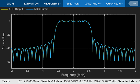
In this same default configuration, the received power spectrum below is noiseless and has no nonlinear distortions. The sidelobes of the spectrum are from the transmit and receive filter responses.
saCfg.OpenAtSimulationStart = true;
cdCfg.OpenAtSimulationStart = false;
cdCfg.Visible = false;
sim(mdl);
The Error Rate Calculation (ERC) block computes the system BER. In the default configuration, with the ERC block discarding transient effects at the beginning of the simulation, the BER is 0.
Exploring the Example
You can investigate multiple RF effects by using the Model Parameters block. By default the Model Parameters block mask default settings applies distortionless values for transmitter IIP3, LNA noise figure, RF Demodulator phase noise, and the ADC number of bits. Typical degraded value levels are shown after the '%' for each of these parameters in the block mask. If you run the simulation with any one of these degraded values set, you will see effects in the constellation, spectrum, and/or BER.
You can reset the following parameters in the Model Parameters block while the simulation is running:
Transmitter IIP3
LNA noise figure
ADC number of bits
ADC full scale voltage
To specify new phase noise values, stop the model first.
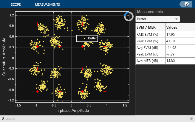
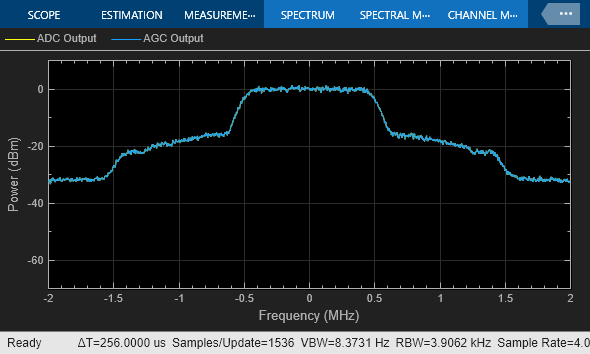
For example, if the transmitter IIP3 is set to 15 dBm, the signal spectrum and constellation diagram show a degraded signal, and the BER degrades to approximately 2.8e-3.
mpBlk = [mdl '/Model Parameters'];
set_param(mpBlk,'txIIP3dBm','15');
cdCfg.OpenAtSimulationStart = true;
cdCfg.Visible = true;
sim(mdl);
You can reset the BER counter while the simulation is running, by double-clicking on the manual switch twice. This is useful to examine the BER effect when you change a parameter value during simulation.
Summary
This example showed how various RF front end impairments, such as amplifier nonlinearities and phase noise, can impact the spectrum, EVM, and BER of a communications system.
close_system(mdl,0)