Memoryless Nonlinearity
Apply amplifier models to complex baseband signal

Libraries:
Communications Toolbox /
RF Impairments and Components
Description
The Memoryless Nonlinearity block applies amplifier models to a complex baseband signal. Use this block to model memoryless nonlinear impairments caused by signal amplification in the radio frequency (RF) transmitter or receiver. For more information, see Memoryless Nonlinear Impairment Models.
Examples
This example applies the Saleh method of memoryless nonlinearity to a 16-QAM modulated signal. To show the Saleh model of a power amplifier, the example applies exaggerated levels that are not typical for modern radios.
The cm_mnl_saleh_16qam model 16-QAM modulates a signal containing a complete set of constellation points and passes them to Memoryless Nonlinearity blocks configured to apply the Saleh method with the default AM/AM and AM/PM distortion settings, AM/AM distortion alone, and AM/PM distortion alone. The model includes Constellation Diagram blocks after each Memoryless Nonlinearity block so you can analyze the impact of each impairment on the constellation.
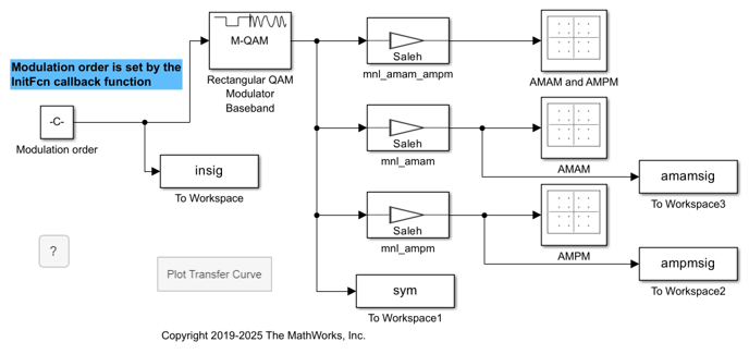
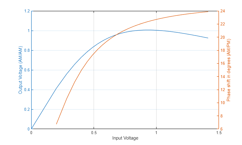
In the model, you can click the Plot Transfer Curve block to run the testPA.m helper function. The testPA helper function plots this amplifier transfer curve for the Saleh method in its default configuration to show the nonlinear input-to-output signal. After amplification, plotted constellation points get displaced according to the input-to-output characteristics of the amplifier model. The voltage for each constellation point determines the direction and magnitude of distortion for each point in the constellation.
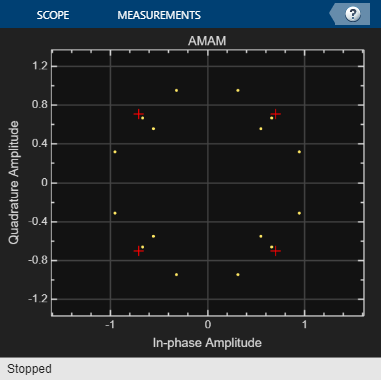
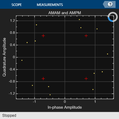
This set of constellation diagrams shows the constellation distortion for the amplifier configured to distort the amplitude and phase individually and together.
The AMAM diagram shows the signal with amplitude-to-amplitude distortion but no amplitude-to-phase distortion. AM/AM distortion displaces constellation points radially away from or toward the origin. For the Saleh method and specified operating characteristics, the inner corner constellation points move away from the origin and the outer corner constellation points move toward the origin. The noncorner constellation points move a negligible amount.
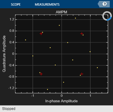
The AMPM diagram shows the signal with amplitude-to-phase distortion but no amplitude-to-amplitude distortion. AM/PM distortion causes rotation of constellation points. Constellation points farther from the origin are more displaced than points closer to the origin.
The AMAM and AMPM diagram shows the signal with amplitude-to-amplitude distortion and amplitude-to-phase distortion. In this diagram, the constellation points move away from or toward the origin and rotate counter-clockwise.

This scatter plot of the constellation points shows points displaced by AM/AM distortion only. The scatterplot function used here plots constellation point locations labeled to highlight the relative distance each point has moved from the ideal constellation point location. To analyze the magnitude and direction each constellation point moved, you would need to replot the input and output characteristic curve for the current operating characteristics.

To explore the model try adjusting settings for the Memoryless Nonlinearity blocks to:
Apply different impairment model methods.
Apply different levels of impairments.
Update the
testPA.mhelper function to plot and analyze input and output characteristics at nondefault Memoryless Nonlinearity block settings.
This example applies RF impairments to a signal modulated by the differential quadrature phase shift keying (DQPSK) method. To show the RF impairments, the example applies exaggerated levels that are not typical levels for modern radios.
In this example, the slex_rcvrimpairments_dqpsk model DQPSK-modulates a random signal and applies various RF impairments to the signal. The model uses impairment blocks from the RF Impairments library. The InitFun callback function initializes simulation variables. For more information, see Model Callbacks (Simulink).
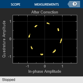
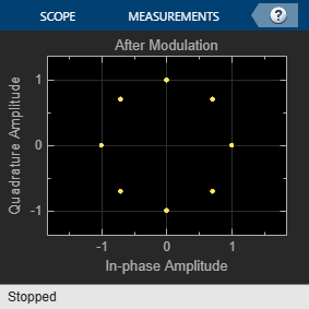
After the impairment blocks, the signal forks into two paths. One path applies DC blocking, automatic gain control (AGC), and I/Q imbalance compensation to the signal before demodulation. The signal on the correction path is adjusted by the DC Blocker, AGC, and I/Q Imbalance Compensator blocks. Because the signal is DQPSK modulated, no carrier synchronization is required. The second path goes directly to demodulation. After demodulation, an error rate calculation is performed on both signals. The model includes Constellation Diagram blocks after modulation, before correction, and after correction so that you can analyze the constellation.
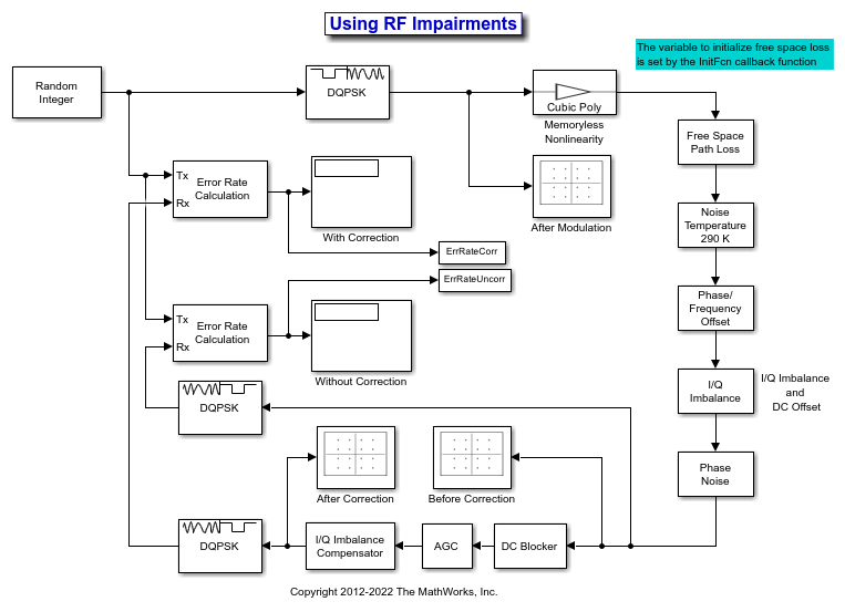
When the model runs, constellation diagrams plot the signal at these stages in the simulation:
The
After Modulationconstellation diagram shows the reference DQPSK-modulated signal constellation.The
Before Correctionconstellation diagram shows the attenuated and distorted signal constellation.The
After Correctionconstellation diagram shows the signal has been amplified and improved after the correction blocks.
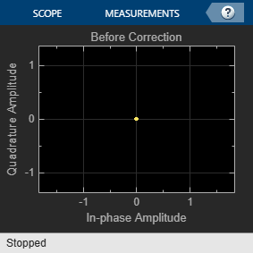
The error rate for the demodulated signal without AGC is primarily caused by free space path loss and I/Q imbalance. The QPSK modulation minimizes the effects of the other impairments.
Error rate for corrected signal:   0.000
Error rate for uncorrected signal: 0.042
To explore the model try:
Adjusting RF impairment settings, rerun the model, and notice the changes to the constellation diagrams and error rates.
Modifying the model to add an equalizer stage before the demodulation. Equalization has inherent ability to reduce some of the distortion caused by impairments. For more information, see Equalization.
Ports
Input
Output
Parameters
Block Characteristics
Data Types |
|
Multidimensional Signals |
|
Variable-Size Signals |
|
More About
Memoryless nonlinear impairments distort the amplitude and phase of the input signal. The amplitude distortion is amplitude-to-amplitude modulation (AM/AM) and the phase distortion is amplitude-to-phase modulation (AM/PM). This block implements these model methods to simulate the memoryless nonlinear impairment models.
| Model Method | Parameter Value | Memoryless Nonlinear Impairment |
|---|---|---|
Cubic polynomial | cubic | Applies AM/AM and AM/PM |
Saleh model | saleh | |
Modified Rapp model | modified-rapp | |
Lookup table | ampm | Applies impairment according to [Pin, Pout, ΔΦ] amplifier characteristics specified by the Lookup table (Pin(dBm), Pout(dBm), deg) parameter |
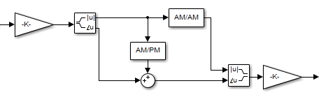
The modeled impairments apply the AM/AM and AM/PM distortions differently according to the model method you specify. The models apply the memoryless nonlinear impairment to the input signal by following these steps.
Multiply the signal by an input gain factor.
Note
You can normalize the signal to 1 by setting the input scaling gain to the inverse of the input signal amplitude.
Split the complex signal into its magnitude and angle components. For real-valued input signals, the imaginary component is set to zero.
Apply an AM/AM distortion to the magnitude of the signal, according to the selected model method, to produce the magnitude of the output signal.
Apply an AM/PM distortion to the phase of the signal, according to the selected model method, to produce the angle of the output signal.
Combine the new magnitude and angle components into a complex signal. Then, multiply the result by an output gain factor.
The model methods apply AM/AM and AM/PM impairments as shown in this figure.
To apply the cubic polynomial model method, set the Model
parameter to cubic. This figure shows the AM/PM
conversion behavior for the cubic polynomial and hyperbolic tangent model
methods.
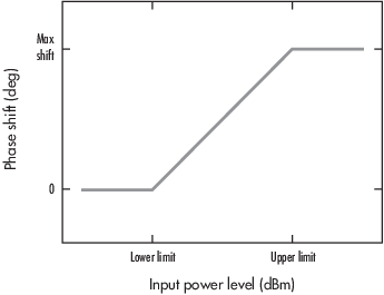
The AM/PM conversion scales linearly with an input power value between the lower and upper limits of the input power level. Outside this range, the AM/PM conversion is constant at the values corresponding to the lower and upper input power limits, which are zero and (AM/PM conversion) × (upper input power limit – lower input power limit), respectively.
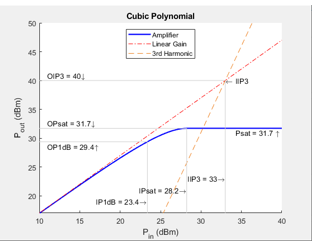
The cubic polynomial method uses linear power gain to determine the linear coefficient of a third-order polynomial and either IP3, P1dB, or Psat to determine the third-order coefficient of the polynomial. The general form of cubic nonlinearity models the AM/AM characteristics as:
where FAM/AM(|u|)
is the magnitude of the output signal, |u| is the magnitude of
the input signal, c1 is the coefficient of
the linear gain term, and c3 is the
coefficient of the cubic gain term. The method takes the results for IIP3, OIP3,
IP1dB, OP1dB, IPsat, and OPsat from [1]. It computes the
c3 coefficient for these nonlinearity
types by using these parameters and equations:
| Parameter | Description | Equation |
|---|---|---|
| IIP3 (dBm) | Input third-order intercept point — Input power level at which the power from linear gain is equal to the power from a third-order nonlinearity |
IIP3 is given in dBm. |
| OIP3 (dBm) | Output third-order intercept point — Output power level at which the power from linear gain is equal to the power from a third-order nonlinearity |
OIP3 is given in dBm. |
| IP1dB (dBm) | Input 1 dB gain compression power — Input power level at which the output power is one dB less than the power from linear gain |
IP1dB is given in dBm. |
| OP1dB (dBm) | Output 1 dB gain compression power — Output power level one dB less than the power from linear gain |
OP1dB is given in dBm, and LGdB is the linear gain in dB. |
| IPsat (dBm) | Input saturation power — Input power at which the output power saturates |
IPsat is given in dBm. |
| OPsat (dBm) | Output saturation power |
OPsat is given in dBm. |
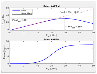
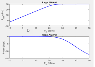
To visualize the power characteristics of your model, set the parameters listed in the table and click the Plot power characteristics button. This table shows power characteristic plot samples for the parameter settings listed in the Parameters and Example Values column.
Model Parameters and Example Values Power Characteristics Plot Cubic Polynomial Main tab:
Linear power gain (dB):
7Type of Non-linearity:
IIP3IIP3 (dBm):
33Simulate using:
Code
                            generation
Saleh Main tab:
Input scaling (dB):
0AM/AM parameters [alpha beta]:
[ 2.1587, 1.1517
												]
AM/PM parameters [alpha beta]:
[ 4.0033, 9.1040
												]
Output scaling (dB):
0Simulate using:
Interpreted
												execution
Modified Rapp Main tab:
Linear power gain (dB):
7Output saturation level (V):
1Magnitude smoothness factor:
2Phase gain (rad):
-.45Phase saturation:
0.88Phase smoothness factor:
3.43Simulate using:
Code generation
Lookup Table Main tab:
Lookup table (Pin(dBm), Pout(dBm), deg):
[-25, 5,
												-1; -10, 20, -2; 0, 27, 5; 5, 28,
												12]
Simulate using:
Code generation

Note
To determine appropriate Pout (dBm) and
degvalues for any Pin (dBm) values below the value specified in the first row of the Lookup table (Pin(dBm), Pout(dBm), deg) parameter, the block applies the same power gain anddegas the first row, to maintain linearity and phase continuity. For any Pin (dBm) higher than the value in the last row of the Lookup table (Pin(dBm), Pout(dBm), deg) parameter, the block uses linear extrapolation from last two rows of the Lookup table (Pin(dBm), Pout(dBm), deg).
References
[1] Kundert, Ken."Accurate and Rapid Measurement of IP2 and IP3," The Designer Guide Community, May 22, 2002.
[2] Saleh, A.A.M. “Frequency-Independent and Frequency-Dependent Nonlinear Models of TWT Amplifiers.” IEEE® Transactions on Communications 29, no. 11 (November 1981): 1715–20. https://doi.org/10.1109/TCOM.1981.1094911.
[3] Rapp, Ch. "Effects of HPA-Nonlinearity on a 4-DPSK/OFDM-Signal for a Digital Sound Broadcasting System." In Proceedings Second European Conf. on Sat. Comm. (ESA SP-332), 179–84. Liege, Belgium, 1991. https://elib.dlr.de/33776/.