comm.MemorylessNonlinearity
Apply memoryless nonlinearity to complex baseband signal
Description
The comm.MemorylessNonlinearity
System object™ applies memoryless nonlinear impairments to a baseband signal. Use this
System object to model memoryless nonlinear impairments caused by signal amplification in a
radio frequency (RF) transmitter or receiver. For more information, see Memoryless Nonlinear Impairment Models.
To apply memoryless nonlinear impairments to a complex baseband signal:
Create the
comm.MemorylessNonlinearityobject and set its properties.Call the object with arguments, as if it were a function.
To learn more about how System objects work, see What Are System Objects?
Creation
Description
mnl = comm.MemorylessNonlinearity
mnl = comm.MemorylessNonlinearity(Name=Value)
Properties
Usage
Syntax
Description
Input Arguments
Output Arguments
Object Functions
To use an object function, specify the
System object as the first input argument. For
example, to release system resources of a System object named obj, use
this syntax:
release(obj)
Examples
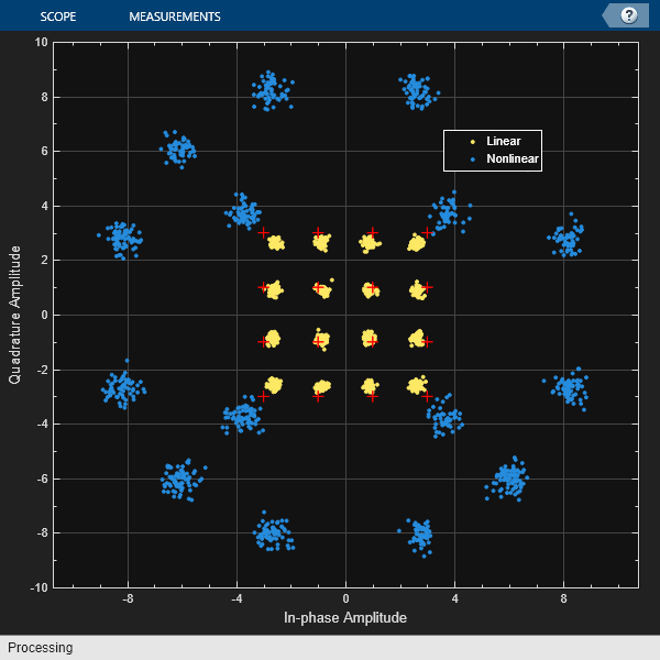
Apply cubic polynomial nonlinearity to two 16-QAM signals. The first input signal power level is in the linear region of the amplifier power characteristic curve. The second input signal power level is in the nonlinear region of the amplifier power characteristic curve. Show the amplifier power characteristic curve and the constellation diagram for the amplified 16-QAM signals.
Initialize Simulation
Initialize variables for simulation and create System objects for a memoryless nonlinearity amplifier impairment and a constellation diagram. So that the constellation shows power compression only (and no phase rotation), configure the memoryless nonlinearity amplifier impairment with AM-PM distortion set to zero.
M = 16; % Modulation order sps = 4; % Samples per symbol pindBm = [12 25]; % Input power gain = 10; % Amplifier gain amplifier = comm.MemorylessNonlinearity(Method="Cubic polynomial", ... LinearGain=gain,ReferenceImpedance=50); refConst = qammod(0:M-1,M); axisLimits = [-gain gain]; constdiag = comm.ConstellationDiagram(NumInputPorts=2, ... ChannelNames=["Linear" "Nonlinear"],ShowLegend=true, ... ReferenceConstellation=refConst, ... XLimits=axisLimits,YLimits=axisLimits);
Amplify and Plot Signal
Apply 16-QAM to an input signal of random data. Amplify the signal and use the plot function of the comm.MemorylessNonlinearity System object to show the output power and phase response curves. The first input signal power level is 12 dBm and is in the linear region of the amplifier power characteristic curve. The second input signal power level is 25 dBm and is in the nonlinear region of the amplifier power characteristic curve.
pin = 10.^((pindBm-30)/10); % Convert dBm to linear Watts
data = randi([0 M-1],1000,1);
modOut = qammod(data,M,UnitAveragePower=true)*sqrt(pin*amplifier.ReferenceImpedance);
ampOut = amplifier(modOut);
plot(amplifier);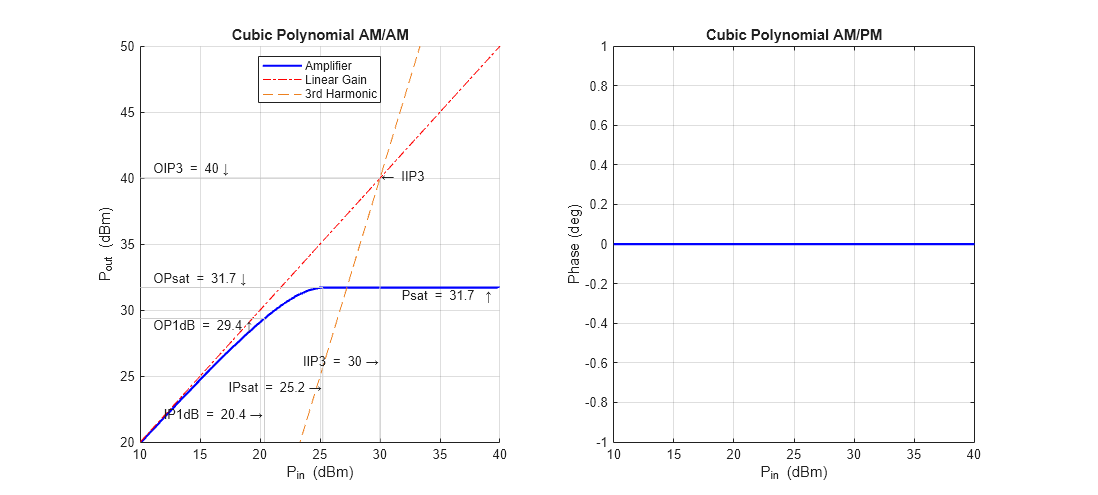
Add AWGN to the two amplified signals and show the constellation diagram for the signals.
snr = 25; noisyLinOut = awgn(ampOut(:,1),snr,"measured"); noisyNonLinOut = awgn(ampOut(:,2),snr,"measured"); constdiag(noisyLinOut,noisyNonLinOut);
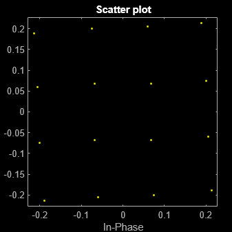
Generate 16-QAM data with an average power of 10 mW and a reference impedance of 1 ohm. Pass the data through a nonlinear power amplifier (PA).
M = 16; data = randi([0 (M - 1)]',1000,1); avgPow = 1e-2; minD = avgPow2MinD(avgPow,M);
Create a memoryless nonlinearity System object, specifying the Saleh model method.
saleh = comm.MemorylessNonlinearity(Method='Saleh model');Generate modulated symbols and pass them through the PA nonlinearity model.
modData = (minD/2).*qammod(data,M); y = saleh(modData);
Generate a scatter plot of the results.
scatterplot(y)
Average power normalization of input signal.
function minD = avgPow2MinD(avgPow,M) % Average power to minimum distance nBits = log2(M); if (mod(nBits,2)==0) % Square QAM sf = (M - 1)/6; else % Cross QAM if (nBits>4) sf = ((31*M/32) - 1)/6; else sf = ((5*M/4) - 1)/6; end end minD = sqrt(avgPow/sf); end
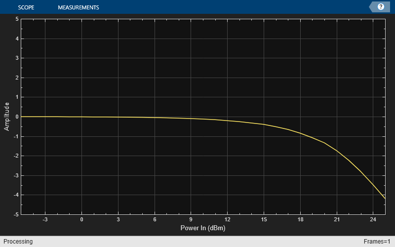
Plot the gain compression of a nonlinear amplifier for a 16-QAM signal.
Specify the modulation order and samples per symbol parameters.
M = 16; sps = 4;
Model a nonlinear amplifier, by creating a memoryless nonlinearity System object with a 30 dB third-order input intercept point. Create a raised cosine transmit filter System object.
amplifier = comm.MemorylessNonlinearity(IIP3=30); txfilter = comm.RaisedCosineTransmitFilter( ... RolloffFactor=0.3,FilterSpanInSymbols=6, ... OutputSamplesPerSymbol=sps,Gain=sqrt(sps));
Specify the input power in dBm and a reference impedance of 1 ohm. Convert the input power to W and initialize the gain vector.
pindBm = -5:25; pin = 10.^((pindBm-30)/10); gain = zeros(length(pindBm),1);
Execute the main processing loop, which includes these steps.
Generate random data symbols.
Modulate the data symbols and adjust the average power of the signal.
Filter the modulated signal.
Amplify the signal.
Measure the gain.
for k = 1:length(pin) data = randi([0 (M - 1)],1000,1); modSig = qammod(data,M,UnitAveragePower=true)*sqrt(pin(k)); filtSig = txfilter(modSig); ampSig = amplifier(filtSig); gain(k) = 10*log10(mean(abs(ampSig).^2) / mean(abs(filtSig).^2)); end
Plot the amplifier gain as a function of the input signal power. The 1 dB gain compression point occurs for an input power of 18.5 dBm. To increase the point at which a 1 dB compression is observed, increase the third-order intercept point, amplifier.IIP3.
arrayplot = dsp.ArrayPlot(PlotType='Line',XLabel='Power In (dBm)', ... XOffset=-5,YLimits=[-5 5]); arrayplot(gain)
Apply nonlinear power amplifier (PA) characteristics with 50 impedance to a 16-QAM signal. Load PA characteristics by setting the Method property to 'Lookup table'. The pa_performance_characteristics helper function outputs the amplifier performance characteristics lookup table.
Define parameters for the modulation order, samples per symbol, and input power. Create random data.
M = 16; % Modulation order sps = 4; % Samples per symbol pindBm = -8; % Input power pin = 10.^((pindBm-30)/10); % power in Watts data = randi([0 (M - 1)],1000,1); refdata = 0:M-1; refconst = qammod(refdata,M,UnitAveragePower=true); paChar = pa_performance_characteristics();
Create a memoryless nonlinearity System object, a transmit filter System object, and a constellation diagram System object. The default lookup table values are used for the memoryless nonlinearity System object.
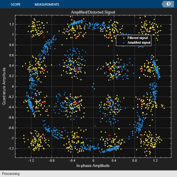
amplifier = comm.MemorylessNonlinearity(Method='Lookup table',Table=paChar,ReferenceImpedance=50); txfilter = comm.RaisedCosineTransmitFilter(RolloffFactor=0.3, ... FilterSpanInSymbols=6,OutputSamplesPerSymbol=sps,Gain=sqrt(sps)); constellation = comm.ConstellationDiagram(SamplesPerSymbol=4, ... Title='Amplified/Distorted Signal',NumInputPorts=2, ... ReferenceConstellation=refconst,ShowLegend=true, ... ChannelNames={'Filtered signal','Amplified signal'});
Modulate the random data. Filter and apply the nonlinear amplifier characteristics to the modulation symbols.
modSig = qammod(data,M,UnitAveragePower=true)*sqrt(pin * amplifier.ReferenceImpedance); filtSig = txfilter(modSig); ampSig = amplifier(filtSig);
Compute input and output signal levels and the phase shift.
pSig = abs(ampSig).^2 / amplifier.ReferenceImpedance; poutdBm = 10 * log10(pSig) + 30; pfiltSig = abs(filtSig).^2 / amplifier.ReferenceImpedance; simulated_pindBm = 10 * log10(pfiltSig) + 30; phase = rad2deg(angle(ampSig.*conj(filtSig)));
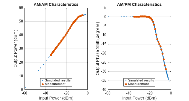
Plot AM/AM characteristics, AM/PM characteristics, and the constellation results.
figure set(gcf,'units','normalized','position',[.25 1/3 .5 1/3]) subplot(1,2,1) plot(simulated_pindBm,poutdBm,'.'); hold on plot(amplifier.Table(:,1),amplifier.Table(:,2),'.',Markersize=15); xlabel('Input Power (dBm)') ylabel('Output Power (dBm)'); grid on; title('AM/AM Characteristics'); leglabel = {'Simulated results','Measurement'}; legend (leglabel,Location='south'); subplot(1,2,2) plot(simulated_pindBm,phase,'.'); hold on plot(amplifier.Table(:,1),amplifier.Table(:,3),'.',Markersize=15); legend (leglabel,Location='south'); xlabel('Input Power (dBm)'); ylabel('Output Phase Shift (degrees)'); grid on; title('AM/PM Characteristics');
For the purpose of constellation comparison, normalize the amplified signal and the filtered signal. Generate a constellation diagram of the filtered signal and amplified signal. The nonlinear amplifier characteristics cause compression of the amplified signal constellation compared to the filtered constellation.
filtSig = filtSig/mean(abs(filtSig)); % Normalized filtered signal ampSig = ampSig/mean(abs(ampSig)); % Normalized amplified signal constellation(filtSig,ampSig)
Helper Function
function paChar = pa_performance_characteristics()The operating specification for the LDMOS-based Doherty amplifier are:
A frequency of 2110 MHz
A peak power of 300 W
A small signal gain of 61 dB
Each row in HAV08_Table specifies Pin (dBm), gain (dB), phase shift (degrees) as derived from figure 4 of Hammi, Oualid, et al. "Power amplifiers' model assessment and memory effects intensity quantification using memoryless post-compensation technique." IEEE Transactions on Microwave Theory and Techniques 56.12 (2008): 3170-3179.
HAV08_Table =...
[-35,60.53,0.01;
-34,60.53,0.01;
-33,60.53,0.08;
-32,60.54,0.08;
-31,60.55,0.1;
-30,60.56,0.08;
-29,60.57,0.14;
-28,60.59,0.19;
-27,60.6,0.23;
-26,60.64,0.21;
-25,60.69,0.28;
-24,60.76,0.21;
-23,60.85,0.12;
-22,60.97,0.08;
-21,61.12,-0.13;
-20,61.31,-0.44;
-19,61.52,-0.94;
-18,61.76,-1.59;
-17,62.01,-2.73;
-16,62.25,-4.31;
-15,62.47,-6.85;
-14,62.56,-9.82;
-13,62.47,-12.29;
-12,62.31,-13.82;
-11,62.2,-15.03;
-10,62.15,-16.27;
-9,62,-18.05;
-8,61.53,-20.21;
-7,60.93,-23.38;
-6,60.2,-26.64;
-5,59.38,-28.75];Convert the second column of the HAV08_Table from gain to Pout for use by the memoryless nonlinearity System object.
paChar = HAV08_Table;
paChar(:,2) = paChar(:,1) + paChar(:,2);
endMore About
Memoryless nonlinear impairments distort the amplitude and phase of the
input signal. The amplitude distortion is amplitude-to-amplitude modulation (AM/AM) and the
phase distortion is amplitude-to-phase modulation (AM/PM). This System object simulates the memoryless nonlinear impairment models listed in this table when
you set the Method property to the value
shown.
| Model Method Property Value | Memoryless Nonlinear Impairment |
|---|---|
'Cubic polynomial' | Applies AM/AM and AM/PM |
'Hyperbolic tangent' | |
'Saleh model' | |
'Ghorbani model' | |
'Modified Rapp model' | |
'Lookup table' | Applies impairment according to
[Pin,
Pout, ΔΦ] amplifier characteristics
specified by the |
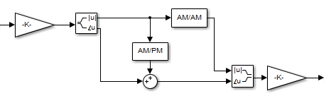
The modeled impairments apply the AM/AM and AM/PM distortions differently according to the model method you specify. The models apply the memoryless nonlinear impairment to the input signal by following these steps.
Multiply the signal by an input gain factor.
Note
You can normalize the signal to 1 by setting the input scaling gain to the inverse of the input signal amplitude.
Split the complex signal into its magnitude and angle components. For real-valued input signals, the imaginary component is set to zero.
Apply an AM/AM distortion to the magnitude of the signal, according to the selected model method, to produce the magnitude of the output signal.
Apply an AM/PM distortion to the phase of the signal, according to the selected model method, to produce the angle of the output signal.
Combine the new magnitude and angle components into a complex signal. Then, multiply the result by an output gain factor.
The model methods apply AM/AM and AM/PM impairments as shown in this figure.
To apply the cubic polynomial or hyperbolic tangent model method, set the Method property to 'Cubic polynomial' or
'Hyperbolic
                tangent'
, respectively. This figure shows the AM/PM
conversion behavior for the cubic polynomial and hyperbolic tangent model methods.
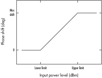
The AM/PM conversion scales linearly with an input power value between the lower and upper limits of the input power level. Outside this range, the AM/PM conversion is constant at the values corresponding to the lower and upper input power limits, which are zero and (AM/PM conversion) × (upper input power limit – lower input power limit), respectively.
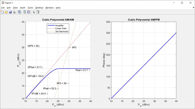
The cubic polynomial method uses linear power gain to determine the linear coefficient of a third-order polynomial and either IP3, P1dB, or Psat to determine the third-order coefficient of the polynomial. The general form of cubic nonlinearity models the AM/AM characteristics as:
where FAM/AM(|u|) is
the magnitude of the output signal, |u| is the magnitude of the input
signal, c1 is the coefficient of the linear gain
term, and c3 is the coefficient of the cubic
gain term. The method takes the results for IIP3, OIP3, IP1dB, OP1dB, IPsat, and OPsat
from [1]. It computes the
c3 coefficient for these nonlinearity types by
using these properties and equations:
| Property | Description | Equation |
|---|---|---|
IIP3 | Input third-order intercept point — Input power level at which the power from linear gain is equal to the power from a third-order nonlinearity | IIP3 is given in dBm. |
OIP3 | Output third-order intercept point — Output power level at which the power from linear gain is equal to the power from a third-order nonlinearity | OIP3 is given in dBm. |
IP1dB | Input 1 dB gain compression power — Input power level at which the output power is one dB less than the power from linear gain | IP1dB is given in dBm. |
OP1dB | Output 1 dB gain compression power — Output power level one dB less than the power from linear gain | OP1dB is given in dBm, and LGdB is the linear gain in dB |
IPsat | Input saturation power — Input power at which the output power saturates | IPsat is given in dBm. |
OPsat | Output saturation power | OPsat is given in dBm. |
This figure shows an example of the plot generated when you set the Method property to 'Cubic polynomial'.
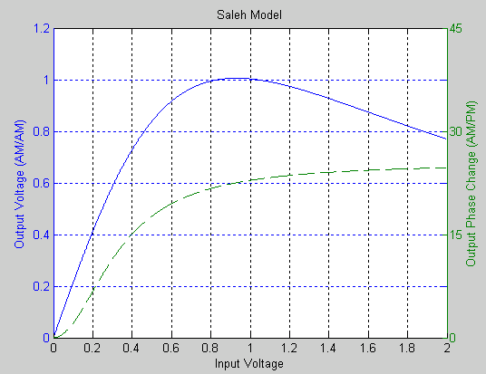
To apply the Saleh model method, set the Method property to 'Saleh model'. As described in [2], the Saleh method is based
on a normalized transfer function and uses input and output scaling parameters to adjust the
signal levels from their normalized values. With the Saleh method,
AMAMParametersspecifies the alphaAM/AM and betaAM/AM variables that compute the amplitude gain for an input signal using this equation:where |u| is the magnitude of the scaled signal and
uis calculated as:AMPMParametersspecifies the alphaAM/PM and betaAM/PM variables that compute the phase change for an input signal using this equation:where |u| is the magnitude of the scaled signal and
angleis a function that returns the phase angle of u.The scaled output signal, uout is calculated as:
This figure shows the AM/AM behavior (output voltage versus input voltage for the AM/AM distortion) and the AM/PM behavior (output phase versus input voltage for the AM/PM distortion) for the Saleh model method.
References
[1] Kundert, Ken."Accurate and Rapid Measurement of IP2 and IP3," The Designer Guide Community, May 22, 2002.
[2] Saleh, A.A.M. “Frequency-Independent and Frequency-Dependent Nonlinear Models of TWT Amplifiers.” IEEE® Transactions on Communications 29, no. 11 (November 1981): 1715–20. https://doi.org/10.1109/TCOM.1981.1094911.
[3] Ghorbani, A., and M. Sheikhan. "The Effect of Solid State Power Amplifiers (SSPAs) Nonlinearities on MPSK and M-QAM Signal Transmission." In 1991 Sixth International Conference on Digital Processing of Signals in Communications (1991): 193–97.
[4] Rapp, Ch. "Effects of HPA-Nonlinearity on a 4-DPSK/OFDM-Signal for a Digital Sound Broadcasting System." In Proceedings Second European Conf. on Sat. Comm. (ESA SP-332), 179–84. Liege, Belgium, 1991. https://elib.dlr.de/33776/.
[5] Choi, C., et.al. "RF impairment models for 60 GHz-band SYS/PHY simulation." IEEE 802.15-06-0477-01-003c. November 2006.
[6] Perahia, E. "TGad Evaluation Methodology." IEEE 802.11-09/0296r16. January 20, 2010. https://mentor.ieee.org/802.11/dcn/09/11-09-0296-16-00ad-evaluation-methodology.doc.