MLSE Equalizers
Maximum-Likelihood Sequence Estimation (MLSE) equalizers provide optimal equalization of time variations in the propagation channel characteristics. However, MLSE equalizers are sometimes less appealing because their computational complexity is higher than Adaptive Equalizers.
In Communications Toolbox™, the mlseeq function, comm.MLSEEqualizer
System object™, and MLSE Equalizer block use the Viterbi algorithm to
equalize a linearly modulated signal through a dispersive channel. These features output the
maximum likelihood sequence estimate of the signal by using an estimate of the channel modeled
as a finite input response (FIR) filter.
To decode a received signal, the MLSE equalizer:
Applies the FIR filter to the symbols in the input signal. The FIR filter tap weights correspond to the channel estimate.
Uses the Viterbi algorithm to compute the traceback paths and the state metric. These values are assigned to the symbols at each step of the Viterbi algorithm. The metrics are based on Euclidean distance.
Outputs the maximum likelihood sequence estimate of the signal as a sequence of complex numbers corresponding to the constellation points of the modulated signal.
An MLSE equalizer yields the best theoretically possible performance, but is computationally intensive.
For background material on MLSE equalizers, see Selected References for Equalizers.
Equalize a Vector Signal in MATLAB
You can use the mlseeq function or comm.MLSEEqualizer
System object for MLSE equalization in MATLAB®. The examples in this section call the mlseeq function. A
similar workflow applies when using the comm.MLSEEqualizer
System object. For examples that use the System object, see the comm.MLSEEqualizer
System object reference page.
The mlseeq function has two operation modes:
Continuous operation mode enables you to process a series of vectors by using repeated calls to
mlseeq. The function saves its internal state information from one call to the next. To learn more, see Equalizing in Continuous Operation Mode.Reset operation mode enables you to specify a preamble and postamble that accompany your data. To learn more, see Using a Preamble or Postamble.
If you are not processing a series of vectors and do not need to specify a preamble or postamble, the operational modes are nearly identical. They differ in that continuous operation mode incurs a delay, while reset operation mode does not. The following example uses reset operation mode. If you modify the example to run using continuous operation mode, there will be delay in the equalized output. To learn more about this delay, see Delays in Continuous Operation Mode.
Use mlseeq to Equalize a Vector Signal
In its simplest form, the mlseeq function equalizes a vector of modulated data when you specify:
The estimated coefficients of the channel (modeled as an FIR filter).
The signal constellation for the modulation type.
The Viterbi algorithm traceback depth. Larger values for the traceback depth can improve the results from the equalizer but increase the computation time.
Generate a PSK modulated signal with modulation order set to four.
M = 4;
msg = pskmod([1 2 2 0 3 1 3 3 2 1 0 2 3 0 1]',M);
Filter the modulated signal through a distortion channel.
chcoeffs = [.986; .845; .237; .12345+.31i];
filtmsg = filter(chcoeffs,1,msg);
Define the reference constellation, traceback length, and channel estimate for the MLSE equalizer. In this example, the exact channel is provided as the channel estimate.
const = pskmod([0:M-1],M);
tblen = 10;
chanest = chcoeffs;
Equalize the received signal.
msgEq = mlseeq(filtmsg,chanest,const,tblen,'rst');
isequal(msg,msgEq)
ans = logical
1
Equalizing Signals in Continuous Operation Mode
If your data is partitioned into a series of vectors (that you process within a loop,
for example), continuous operation mode is an appropriate way to use the
mlseeq function. In continuous operation mode,
mlseeq can save its internal state information for use in a
subsequent invocation and can initialize by using previously stored state information. To
choose continuous operation mode when invoking mlseeq, specify
'cont' as an input argument.
Note
Continuous operation mode incurs a delay, as described in Delays in Continuous Operation Mode. This mode cannot accommodate a preamble or postamble.
Procedure for Continuous Operation Mode
When using continuous operation mode within a loop, preallocate three empty matrix
variables to store the state metrics, traceback states, and traceback inputs for the
equalizer before the equalization loop starts. Inside the loop, invoke
mlseeq using a syntax such
as:
sm = [];
ts = [];
ti = [];
for ...
    [y,sm,ts,ti] = mlseeq(x,chcoeffs,const,tblen,'cont',nsamp,sm,ts,ti);
...
end
Using sm, ts, and ti as input
arguments causes mlseeq to continue operating from where it finished
in the previous iteration. Using sm, ts, and
ti as output arguments causes mlseeq to update
the state information at the end of the current iteration. In the first iteration,
sm, ts, and ti start as empty
matrices, so the first invocation of the mlseeq function initializes
the metrics of all states to 0.
Delays in Continuous Operation Mode
Continuous operation mode with a traceback depth of tblen incurs an
output delay of tblen symbols. The first tblen
output symbols are unrelated to the input signal and the last tblen
input symbols are unrelated to the output signal. For example, this command uses a
traceback depth of 3. The first three output symbols are unrelated to
the input signal of ones(1,10).
y = mlseeq(ones(1,10),1,[-7:2:7],3,'cont')y =
-7 -7 -7 1 1 1 1 1 1 1
It is important to keep track of delays introduced by different portions of the communications system. The Use mlseeq to Equalize a Vector in Continuous Operation Mode example illustrates how to account for the delay when computing an error rate.
Use mlseeq to Equalize a Vector in Continuous Operation Mode
This example shows the procedure for using the continuous operation mode of the mlseeq function within a loop.
Initialize Variables
Specify run-time variables.
numsym = 200; % Number of symbols in each iteration
numiter = 25; % Number of iterations

M = 4; % Use QPSK modulation

chcoeffs = [1 ; 0.25]; % Channel coefficients
chanest = chcoeffs; % Channel estimate
To initialize the equalizer, define parameters for the reference constellation, traceback length, number of samples per symbol, and the state variables sm, ts, and ti.
const = pskmod((0:M-1)',M);
tblen = 10;
nsamp = 1;
sm = [];
ts = [];
ti = [];
Define and preallocate variables to accumulate results from each iteration of the loop.
fullmodmsg = [zeros(numiter*numsym,1)];
fullfiltmsg = [zeros(size(fullmodmsg))];
fullrx = [zeros(size(fullmodmsg))];
Simulate the System by Using a Loop
Run the simulation in a loop that generates random data, modulates the data by using baseband QPSK modulation, and filters the data. The mlseeq function equalizes the filtered data. The loop also updates the variables that accumulate results from each iteration of the loop.
for jj = 1:numiter
    msg = randi([0 M-1],numsym,1); % Random signal vector
    modmsg = pskmod(msg,M); % QPSK-modulated signal
    filtmsg = filter(chcoeffs,1,modmsg); % Filtered signal
    % Equalize the signal.
    [rx,sm,ts,ti] = mlseeq(filtmsg,chanest,const, ...
        tblen,'cont',nsamp,sm,ts,ti);
    % Update vectors with cumulative results.
    fullmodmsg = [fullmodmsg; modmsg];
    fullfiltmsg = [fullfiltmsg; filtmsg];
    fullrx = [fullrx; rx];
end
Computing an Error Rate and Plotting Results
Compute the symbol error rate from all iterations of the loop. The symerr function compares selected portions of the received and transmitted signals, not the entire signals. Because continuous operation mode incurs a delay whose length in samples is the traceback depth (tblen) of the equalizer, exclude the first tblen samples from the received signal and the last tblen samples from the transmitted signal. Excluding samples that represent the delay of the equalizer ensures that the symbol error rate calculation compares samples from the received and transmitted signals that are meaningful and that truly correspond to each other.
Taking the delay into account, compute the total number of symbol errors.
hErrorCalc = comm.ErrorRate(ReceiveDelay=10);
err = hErrorCalc(fullmodmsg,fullrx);
numsymerrs = err(1)
numsymerrs =
0.0010
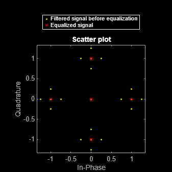
Plot the signal constellation before and after equalization. The points in the equalized signal coincide with the points of the ideal signal constellation for QPSK.
h = scatterplot(fullfiltmsg);
hold on;
scatterplot(fullrx,1,0,'r*',h);
legend('Filtered signal before equalization', ...
    'Equalized signal', ...
   Location='NorthOutside');
hold off;
Use a Preamble or a Postamble
Some systems include a sequence of known symbols at the beginning or end of a set of
data. The known sequence at the beginning or end is called a preamble
or postamble, respectively. The mlseeq function
can accommodate a preamble and postamble that are already incorporated into its input
signal. When you invoke the function, you specify the preamble and postamble as integer
vectors that represent the sequence of known symbols by indexing into the signal
constellation vector. For example, a preamble vector of [1 4 4] and a
4-PSK signal constellation of [1 j -1 -j] indicates that the modulated
signal begins with [1 -j -j].
If your system uses a preamble without a postamble, use a postamble vector of
[] when invoking mlseeq. If your system uses a
postamble without a preamble, use a preamble vector of [].
Recover Message Containing Preamble
Recover a message that includes a preamble, equalize the signal, and check the symbol error rate.
Specify the modulation order, equalizer traceback depth, number of samples per symbol, preamble, and message length.
M = 4;
tblen = 16;
nsamp = 1;
preamble = [3;1];
msgLen = 500;
Generate the reference constellation.
const = pskmod(0:3,4);
Generate a message by using random data and prepend the preamble to the message. Modulate the random data.
msgData = randi([0 M-1],msgLen,1);
msgData = [preamble; msgData];
msgSym = pskmod(msgData,M);
Filter the data through a distortion channel and add Gaussian noise to the signal.
chcoeffs = [0.623; 0.489+0.234i; 0.398i; 0.21];
chanest = chcoeffs;
msgFilt = filter(chcoeffs,1,msgSym);
msgRx = awgn(msgFilt,9,'measured');
Equalize the received signal. To configure the equalizer, provide the channel estimate, reference constellation, equalizer traceback depth, operating mode, number of samples per symbol, and preamble. The same preamble symbols appear at the beginning of the message vector and in the syntax for mlseeq. Because the system does not use a postamble, an empty vector is specified as the last input argument in this mlseeq syntax.
Check the symbol error rate of the equalized signal. Run-to-run results vary due to use of random numbers.
eqSym = mlseeq(msgRx,chanest,const,tblen,'rst',nsamp,preamble,[]);
[nsymerrs,ser] = symerr(msgSym,eqSym)
nsymerrs = 7
ser =
0.0139
Using MLSE Equalizers in Simulink
The MLSE Equalizer block uses the Viterbi algorithm to equalize a linearly modulated signal through a dispersive channel. The block outputs the maximum likelihood sequence estimate (MLSE) of the signal by using your estimate of the channel modeled as a finite input response (FIR) filter. When using the MLSE Equalizer block, you specify the channel estimate and the signal constellation of the input signal. You can also specify an expected input signal preamble and postamble as input parameters to the MLSE Equalizer block.
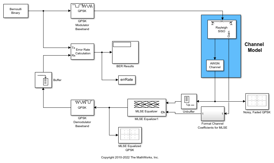
MLSE Equalization with Dynamically Changing Channel
Use a Maximum Likelihood Sequence Estimation (MLSE) equalizer to equalize the effects of a multipath Rayleigh fading channel. The MLSE equalizer inputs data that has passed through a time varying dispersive channel and an estimate of the channel. The channel estimate contains dynamically evolving channel coefficients of a two-path Rayleigh fading channel.
Model Structure
The transmitter generates QPSK random signal data.
Channel impairments include multipath fading and AWGN.
The receiver applies MLSE equalization and QPSK demodulation.
The model uses scopes and a BER calculation to show the system behavior.
Explore Example Model
Experimenting with the model
The Bernoulli Binary Generator block sample time of 5e-6 seconds corresponds to a bit rate of 200 kbps and a QPSK symbol rate of 100 ksym/sec.
The Multipath Rayleigh Fading Channel block settings are:
Maximum Doppler shift is 30 Hz.
Discrete path delay is [0 1e-5], which corresponds to two consecutive sample times of the input QPSK symbol data. This delay reflects the simplest delay vector for a two-path channel.
Average path gain is [0 -10].
Average path gains are normalized to 0 dB so that the average power input to the
AWGNblock is 1 W.
The MLSE Equalizer block has the Traceback depth set to 10. Vary this depth to study its effect on Bit Error rate (BER).
The QPSK demodulator accepts an N-by-1 input frame and generates a 2N-by-1 output frame. This output frame and a traceback depth of 10 results in a delay of 20 bits. The model performs frame-based processing on frames that have 100 samples per frame. Due to the frame-based processing, there is an inherent delay of 100 bits in the model. The combined receive delay of 120 is set in the Receive delay parameter of the Error Rate Calculation block, aligning the samples.
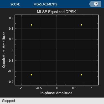
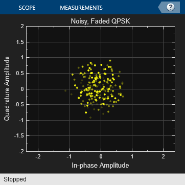
The computed BER is displayed. Constellation plots show the constellation before and after equalization.
BER = 0.033508