Simulate and Verify Power Amplifier Backoff
This example shows how to use backoff to scale a signal prior to inputting it to a table-based power amplifier. It also shows how to examine the power distribution of the signal input to the amplifier, and to verify that the actual behavior of the amplifier matches the specification. The Appendix lists helper functions used in the example.
System Setup
M = 16;             % Modulation order
fs = 1e6;           % Sample rate in Hz & measurement bandwidth
sigDuration = 0.01; % seconds
msgLen = round(sigDuration*fs); % Number of samples
totalTime = 0;
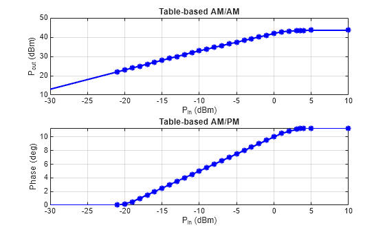
Specify the amplifier as a table-based object. Using measured amplifier data stored in an Excel spreadsheet, read the output power vs. input power and phase change vs. input power. The powers are given in dBm, and the phase change in degrees. The reference impedance is used to convert the signal's voltage values to power values.
table = table2array(readtable( ...
    "PACharacteristic.xlsx", ...
    PreserveVariableNames=true));
mnl = comm.MemorylessNonlinearity( ...
    Method="Lookup table", ...
    Table=table, ...
    ReferenceImpedance=1);
Determine the input power that results in the peak output power. That input power is the point from which the signal will be backed off. Use the input backoff to determine the required signal power at the input to the amplifier.
[pkOpPwr, idxPk] = max(mnl.Table(:, 2)); % dBm
ipPwrAtPkOut = mnl.Table(idxPk, 1);      % dBm
IBO = 6;                                 % input backoff set point, dB
rqdIpPwr = ipPwrAtPkOut - IBO;           % dBm
Plot AM/AM and AM/PM amplifier characteristics. The plotted values match those in the spreadsheet.
plot(mnl);
System Simulation and Verification
Create a raised cosine transmit filter System object™ for pulse shaping.
txFilt = comm.RaisedCosineTransmitFilter( ...
  Shape='Square root', ...
  RolloffFactor=0.2, ...
  FilterSpanInSymbols=10, ...
  OutputSamplesPerSymbol=4);
Create a power meter System object to measure power at multiple points in the processing chain. Set the measurement window of the power meter to 10 ms.
pm = powermeter(...
  Measurement="Average power", ...
  WindowLength=round(sigDuration*fs), ...
  ReferenceLoad=mnl.ReferenceImpedance, ...
  PowerUnits="dBm");
Generate a modulated signal, filter it, scale it to -10 dBm, and measure powers. The filtered signal is roughly constant amplitude throughout its duration, so the power measurement window can extend over the entire duration.
filtTransient = ...
    txFilt.FilterSpanInSymbols*txFilt.OutputSamplesPerSymbol;
msg = randi([0 M-1],msgLen+filtTransient,1);
modOut = qammod(msg,M, ...
    UnitAveragePower=true);             % 0 dBW (30 dBm)
filtOut = txFilt(modOut);
filtOut = filtOut(1+filtTransient:end); % Truncate beginning transient
PFiltOutdBm = pm(filtOut);
Pdesired = -10;  % dBm
scaleFactor = 10.^((Pdesired - PFiltOutdBm(end))/20);
filtOut = scaleFactor * filtOut;
reset(pm);
PFiltOutdBm = pm(filtOut);
fprintf('The filtered, scaled signal power is %4.2f dBm.\n', ...
    PFiltOutdBm(end))
The filtered, scaled signal power is -10.00 dBm.
PFiltOutdBW = PFiltOutdBm(end) - 30;
Scale the amplifier input power to the desired backoff. The measured power of the backed off signal must be equal to the input power at peak output (5 dBm) less the input backoff (6 dB). The power meter verifies that the signal has been properly backed off.
gain = helperBackoffGain(ipPwrAtPkOut,PFiltOutdBm(end),IBO);
ampIn = gain * filtOut;
reset(pm);
PAmpIndBm = pm(ampIn);
fprintf('The backed off signal power is %4.2f dBm.\n', ...
    PAmpIndBm(end))
The backed off signal power is -1.00 dBm.
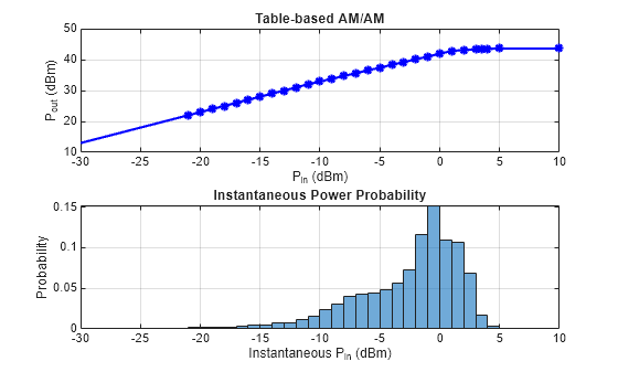
Plot a histogram of instantaneous input power into the amplifier. The following figure shows that a significant percentage of the amplifier input samples have a power that should cause gain compression at the amplifier output. Many signal samples have powers above 0 dBm, where the amplifier behaves nonlinearly.
PAmpInInst = abs(ampIn).^2 / mnl.ReferenceImpedance;
PAmpInInstdBm = 10*log10(PAmpInInst) + 30;
edges = -29:9;
histogram(PAmpInInstdBm,edges,Normalization="probability")
title("Instantaneous Power Probability");
xlabel("Instantaneous P_i_n (dBm)");
ylabel("Probability");
xlim([-30 10]);
grid on;
Pass the signal through the amplifier. The measured average power at the amplifier output closely corresponds to the expected instantaneous power illustrated by the previous figure.
ampOut = mnl(ampIn);
PAmpOutdBm = pm(ampOut);
fprintf('The amplifier output power is %4.2f dBm.\n', ...
    PAmpOutdBm(end))
The amplifier output power is 40.63 dBm.
Calculate average amplifier gain.
ampGaindB = PAmpOutdBm(end) - PAmpIndBm(end);
fprintf('The amplifier gain is %4.2f dB.\n', ...
    ampGaindB)
The amplifier gain is 41.63 dB.
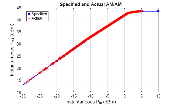
Plot the specified and actual instantaneous vs. to show that the actual behavior of the amplifier matches the behavior specified by the table-based object.
figure;
hFig = helperPlotAMAM(mnl); % Specified Pout vs. Pin
hold on;
pAmpOutInst = abs(ampOut).^2 / mnl.ReferenceImpedance;
pAmpOutInstdBm = 10*log10(pAmpOutInst) + 30;  % Actual Pout vs Pin
plot(PAmpInInstdBm,pAmpOutInstdBm,'r*');
grid on;
lines = hFig.Children.Children;
legend(lines([2 1]),Specified="Actual",Location="Northwest");
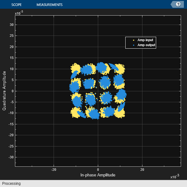
Create a constellation diagram to illustrate the amplifier input and output signals. The constellation diagram of the 16QAM constellation shows the amplifier output has been slightly rotated (AM/PM distortion), and the corner points have incurred some gain compression (AM/AM distortion).
constDiag = comm.ConstellationDiagram( ...
  ShowReferenceConstellation=false, ...
  SamplesPerSymbol=txFilt.OutputSamplesPerSymbol, ...
  ShowLegend=true, ...
  ChannelNames={'Amp input','Amp output'});

% Set plot limits
maxLim = 2 * max(real(filtOut));
constDiag.XLimits = [-maxLim maxLim];
constDiag.YLimits = [-maxLim maxLim];

magFiltOut = sqrt(mean(abs(filtOut).^2));
magAmpOut = sqrt(mean(abs(ampOut).^2));
gain = magAmpOut / magFiltOut;
constDiag([filtOut,ampOut/gain]); % Scale amp output for plotting ease
Exploring the Example
You can experiment with the example by trying different backoff levels or modulated signals (for example, 64QAM or OFDM). You can load a spreadsheet with your own table-based characteristics to apply this backoff technique to your PA characterization.
Summary
This example demonstrated how to apply backoff to the input signal of a nonlinear amplifier. The technique was verified by comparing behavior of the specified and actual data.
Appendix
These helper files are used in the example:
helperBackoffGain.m
helperPlotAMAM.m