Model Reduction in the Live Editor
This example shows how to use the Reduce Model Order task in the Live Editor to generate code for performing model reduction by balanced truncation, mode selection, and pole-zero simplification. The Reduce Model Order task lets you interactively compute reduced-order approximations of high-order models while preserving model characteristics that are important to your application.
Open this example to see a preconfigured script containing the Reduce Model Order task. For more information about Live Editor tasks generally, see Add Interactive Tasks to a Live Script.
In the Live Editor, load the model you want to reduce into the MATLAB® workspace.
load build G
size(G)
State-space model with 1 outputs, 1 inputs, and 48 states.
The LTI model G is a state-space model with 48 states. Some of these states can be discarded while preserving relevant dynamics. To experiment with reducing the model, open the Reduce Model Order Live Editor task. On the Live Editor tab, select Task > Reduce Model Order.
Balanced Truncation
Balanced truncation computes a lower-order approximation of your model by removing states with relatively small energy contributions. For more information about balanced truncation, see Balanced Truncation Model Reduction.
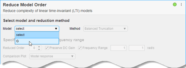
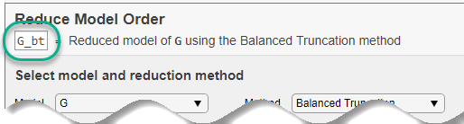
To generate code for balanced truncation in the Reduce Model Order task, select G as the model to reduce. Specify Balanced Truncation as the Method.
Specify the target Reduced Order of the reduced model. You can use the Hankel singular-value plot to help select a target order. This plot visualizes the relative energy contribution of each state in the original model. The task discards states with lower energy than the state you select in this plot.
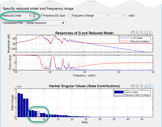
The response plot shows the Bode plot of the original model and the reduced-order model. Experiment with different reduced-order models by selecting different orders on the Hankel singular-value plot, using the response plot to observe how the reduced-order model changes. (To see the absolute or relative error between the original and reduced model, use the Model Response menu.)
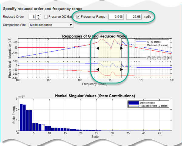
Select the smallest model order that adequately preserves the dynamics that are important to your application. If you are only interested in dynamics in a specific frequency range, you can restrict the computation of energy contributions to that range. To do, select Frequency Range. Then, enter the minimum and maximum frequencies or specify the range using the vertical sliders on the response plot. (Selecting Frequency Range clears the Preserve DC Gain option, because 0 rad/s is not within the default frequency range.)
The task generates the code to compute the reduced model that you have specified. To see the generated code, click ![]() Show code at the bottom of the task. The task expands to show the generated code. For balanced truncation, Reduce Model Order uses
Show code at the bottom of the task. The task expands to show the generated code. For balanced truncation, Reduce Model Order uses reducespec with method set to "balanced". (To include code that produces a response plot, in the Output Plot menu, select the response you want.)
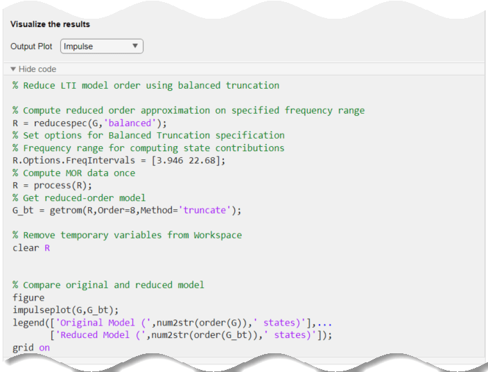
By default, the generated code uses G_bt as the name of the output variable. To specify a different output variable name, enter a new name in the summary line at the top of the task.
The task updates the generated code to reflect the new variable, and a reduced-order state-space model appears in the MATLAB® workspace with the new name.
Mode Selection
You can use the reduced-order model in the MATLAB workspace as you would use any other LTI model for analysis and control design. For this example, compare the reduced model responses to a reduced-order model created using a different model-reduction method, mode selection. Mode selection reduces the model by discarding dynamics that fall outside a frequency region you specify.
Change the name of the output variable to G_mr, so you do not overwrite the model you created using balanced truncation. Then, set the reduction method to Mode Selection. Use the vertical sliders on the plot to choose the frequency range within which to preserve dynamics, or enter the frequency range in Cutoff Frequency.
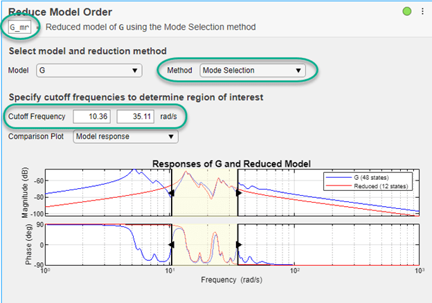
For mode selection, Reduce Model Order generates code that uses reducespec with "modal" method. It can be useful to add a pole-zero plot to observe which poles and zeros are eliminated from the reduced-order model. To do so, in the Output Plot menu, select Pole-Zero. This selection generates a plot that shows the poles and zeros of both the original and reduced model. It also adds the code for creating that plot to the generated code.
Pole-Zero Simplification
Pole-zero simplification reduces the order of your model exactly by canceling pole-zero pairs or eliminating states that have no effect on the overall model response. Pole-zero pairs can be introduced, for example, when you construct closed-loop architectures. Normal small errors associated with numerical computation can convert such canceling pairs to near-canceling pairs. Removing these states preserves the model response characteristics while simplifying analysis and control design.
The Pole-Zero Simplification method of Reduce Model Order automatically eliminates:
Canceling or near-canceling pole-zero pairs from transfer functions
Unobservable or uncontrollable states from state-space models
States that are structurally disconnected from the inputs or outputs.
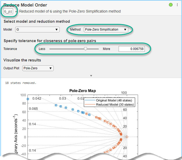
Change the name of the output variable to G_pz, so you do not overwrite the model you created using the other methods. Then, set the reduction method to Pole-Zero Cancellation. Use the Tolerance parameter to adjust how close to canceling pole-zero pairs must be to be eliminated. Move the slider toward More to cancel more pole-zero pairs, reducing the model to a smaller order. In Output Plot, select Pole-Zero and use the plot to observe which poles and zeros are eliminated from the reduced model.
Use Reduced-Order Models
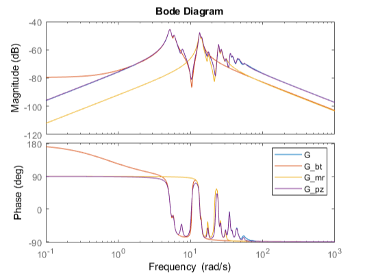
The Reduce Model Order task creates the reduced-order models in the MATLAB workspace automatically. You can use those models for further analysis or control design as you would use any other LTI model. For instance, compare the frequency responses of the original and all reduced-order models on one plot.
bode(G,G_bt,G_mr,G_pz,{0.1,1000})
legend