Plant Models for Gain-Scheduled Controller Tuning
Gain scheduling is a control approach for controlling a nonlinear plant. To tune a gain-scheduled control system, you need a collection of linear models that approximate the nonlinear dynamics near selected design points. Generally, the dynamics of the plant are described by nonlinear differential equations of the form:
Here, x is the state vector, u is the plant input, and y is the plant output. These nonlinear differential equations can be known explicitly for a particular system. More commonly, they are specified implicitly, such as by a Simulink® model.
You can convert these nonlinear dynamics into a family of linear models that describe the local behavior of the plant around a family of operating points (x(σ),u(σ)), parameterized by the scheduling variables, σ. Deviations from the nominal operating condition are defined as:
These deviations are governed, to first order, by linear parameter-varying dynamics:
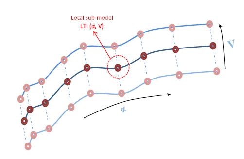
This continuum of linear approximations to the nonlinear dynamics is called a linear parameter-varying (LPV) model:
The LPV model describes how the linearized plant dynamics vary with time, operating condition, or any other scheduling variable. For example, the pitch axis dynamics of an aircraft can be approximated by an LPV model that depends on incidence angle, α, air speed, V, and altitude, h.
In practice, you replace this continuum of plant models by a finite set of linear models obtained for a suitable grid of σ values This replacement amounts to sampling the LPV dynamics over the operating range and selecting a representative set of σ values, your design points.
Gain-scheduled controllers yield best results when the plant dynamics vary smoothly between design points.
Obtaining the Family of Linear Models
If you do not have this family of linear models, there are several approaches to obtaining it, including:
If you have a Simulink model, trim and linearize the model at the design points.
Linearize the Simulink model using parameter variation.
If the scheduling variable is time, linearize the model at a series of simulation snapshots.
If you have nonlinear differential equations that describe the plant, linearize them at the design points.
For tuning gain schedules, after you obtain the family of linear models, you must
associate it with an slTuner interface to build a family of tunable
closed-loop models. To do so, use block substitution, as described in Multiple Design Points in slTuner Interface.
Set Up for Gain Scheduling by Linearizing at Design Points
This example shows how to linearize a plant model at a set of design points for tuning of a gain-scheduled controller. The example then uses the resulting linearized models to configure an slTuner interface for tuning the gain schedule.
Open the rct_CSTR model.
mdl = "rct_CSTR";
open_system(mdl)
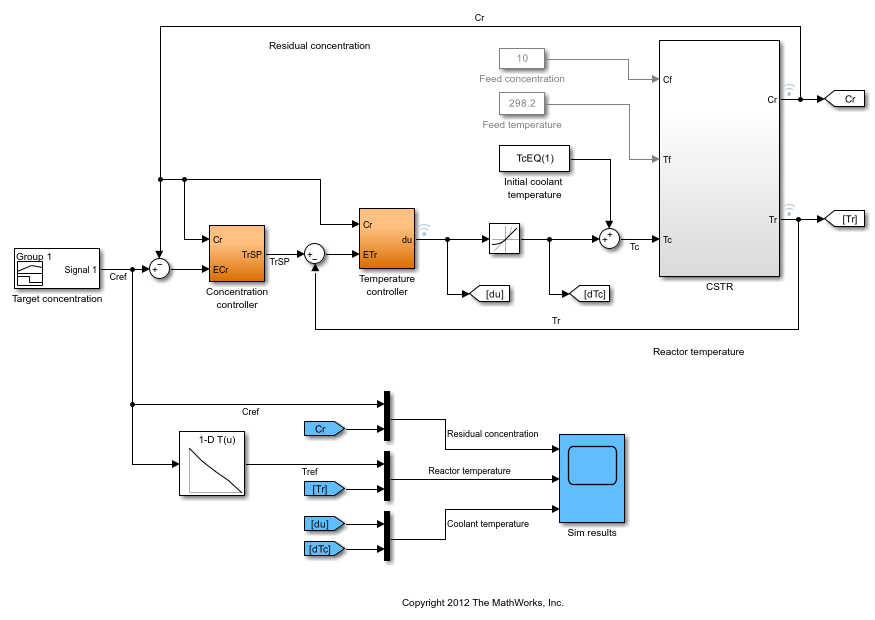
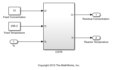
In this model, the Concentration controller and Temperature controller both depend on the output concentration Cr. To set up this gain-scheduled system for tuning, you linearize the plant at a set of steady-state operating points that correspond to different values of the scheduling parameter Cr. Sometimes, it is convenient to use a separate model of the plant for trimming and linearization under various operating conditions. For example, in this case, the most straightforward way to obtain these linearizations is to use a separate open-loop model of the plant, rct_CSTR_OL.
mdl_OL = "rct_CSTR_OL";
open_system(mdl_OL)
Trim Plant at Design Points
Suppose that you want to control this plant at a range of Cr values from 4 to 8. Trim the model to find steady-state operating points for a set of values in this range. These values are the design points for tuning.
Cr = (4:8)';        % concentrations
for k=1:length(Cr)
   opspec = operspec(mdl_OL);
   % Set desired residual concentration
   opspec.Outputs(1).y = Cr(k);
   opspec.Outputs(1).Known = true;
   % Compute equilibrium condition
   opt = findopOptions(DisplayReport="off");
   [op(k),report(k)] = findop(mdl_OL,opspec,opt);
end
op is an array of steady-state operating points. For more information about steady-state operating points, see About Operating Points (Simulink Control Design).
Linearize at Design Points
Linearizing the plant model using op returns an array of LTI models, each linearized at the corresponding design point.
G = linearize(mdl_OL,"rct_CSTR_OL/CSTR",op);
Create slTuner Interface with Block Substitution
To tune the control system rct_CSTR, create an slTuner interface that linearizes the system at those design points. Use block substitution to replace the plant in rct_CSTR with the linearized plant-model array G.
blocksub.Name = "rct_CSTR/CSTR";
blocksub.Value = G;
tunedblocks = {'Kp','Ki'};
ST0 = slTuner(mdl,tunedblocks,blocksub);
For this example, only the PI coefficients in the Concentration controller are designated as tuned blocks. In general, however, tunedblocks lists all the blocks to tune.
For more information about using block substitution to configure an slTuner interface for gain-scheduled controller tuning, see Multiple Design Points in slTuner Interface.
For another example that illustrates using trimming and linearization to generate a family of linear models for gain-scheduled controller tuning, see Trimming and Linearization of the HL-20 Airframe.
Sample System at Simulation Snapshots
If you are controlling the system around a reference trajectory (x(σ),u(σ)), use snapshot linearization to sample the system at various points along the σ trajectory. Use this approach for time-varying systems where the scheduling variable is time.
To linearize a system at a set of simulation snapshots, use a vector of positive scalars
as the op input argument of linearize,
slLinearizer, or slTuner. These scalars are the
simulation times at which to linearize the model. Use the same set of time values as the
design points in tunable surfaces for the system.
Sample System at Varying Parameter Values
If the scheduling variable is a parameter in the Simulink model, you can use parameter variation to sample the control system over a
parameter grid. For example, suppose that you want to tune a model named
suspension_gs that contains two parameters, Ks and
Bs. These parameters each can vary over some known range, and a
controller gain in the model varies as a function of both parameters.
To set up such a model for tuning, create a grid of parameter values. For this example,
let Ks vary from 1 – 5, and let Bs vary from 0.6 –
0.9.
Ks = 1:5;
Bs = [0.6:0.1:0.9];
[Ksgrid,Bsgrid] = ndgrid(Ks,Bs);
These values are the design points at which to sample and tune the system. For example,
create an slTuner interface to the model, assuming one tunable block, a
Lookup Table block named K that models the
parameter-dependent gain.
params(1) = struct('Name','Ks','Value',Ksgrid);
params(2) = struct('Name','Bs','Value',Bsgrid);
STO = slTuner('suspension_gs','K',params);
slTuner samples the model at all (Ksgrid,Bsgrid)
values specified in params.
Next, use the same design points to create a tunable gain surface for parameterizing
K.
design = struct('Ks',Ksgrid,'Bs',Bsgrid);
shapefcn = @(Ks,Bs)[Ks,Bs,Ks*Bs];
K = tunableSurface('K',1,design,shapefcn);
setBlockParam(ST0,'K',K);
After you parameterize all the scheduled gains, you can create your tuning goals and
tune the system with systune.
Eliminate Samples at Unneeded Design Points
Sometimes, your sampling grid includes points that represent irrelevant or unphysical
design points. You can eliminate such design points from the model grid entirely, so that
they do not contribute to any stage of tuning or analysis. To do so, use voidModel,
which replaces specified models in a model array with NaN.
voidModel replaces specified models in a model array with
NaN. Using voidModel lets your design over a grid
of design points that is almost regular.
There are other tools for controlling which models contribute to design and analysis. For instance, you might want to:
Keep a model in the grid for analysis, but exclude it from tuning.
Keep a model in the grid for tuning, but exclude it from a particular design goal.
For more information, see Change Requirements with Operating Condition.
LPV Plants in MATLAB
In MATLAB®, you can use an array of LTI plant models to represent an LPV system sampled
at varying values of σ. To associate each linear model in the set with
the underlying design points, use the SamplingGrid property of the LTI
model array σ. One way to obtain such an array is to create a parametric
generalized state-space (genss) model of the system and sample the
model with parameter variation to generate the array. For an example, see Study Parameter Variation by Sampling Tunable Model.
See Also
slTuner (Simulink Control Design) | findop (Simulink Control Design) | voidModel