Custom Nonlinear Census Fitting
This example shows how to fit a custom equation to census data, specifying bounds, coefficients, and a problem-dependent parameter.
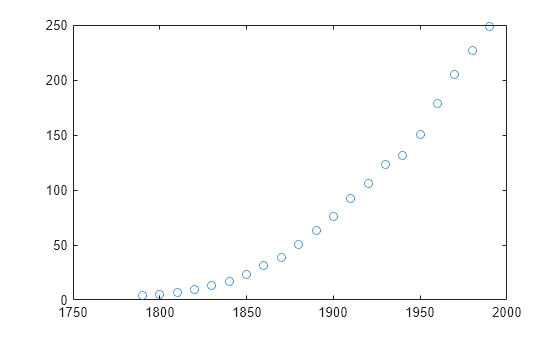
Load and plot the data in census.mat:
load census
plot(cdate,pop,'o')
hold on
Create a fitoptions object and a fittype object for the custom nonlinear model, where a and b are coefficients and n is a problem-dependent parameter. See the fittype function page for more details on problem-dependent parameters.
s = fitoptions('Method','NonlinearLeastSquares',...
               'Lower',[0,0],...
               'Upper',[Inf,max(cdate)],...
               'Startpoint',[1 1]);
f = fittype('a*(x-b)^n','problem','n','options',s);
Fit the data using the fit options and a value of n = 2:
[c2,gof2] = fit(cdate,pop,f,'problem',2)c2 =
General model:
c2(x) = a*(x-b)^n
Coefficients (with 95% confidence bounds):
a = 0.006092 (0.005743, 0.006441)
b = 1789 (1784, 1793)
Problem parameters:
n = 2
gof2 = struct with fields:
           sse: 246.1543
       rsquare: 0.9980
           dfe: 19
    adjrsquare: 0.9979
          rmse: 3.5994
Fit the data using the fit options and a value of n = 3:
[c3,gof3] = fit(cdate,pop,f,'problem',3)c3 =
General model:
c3(x) = a*(x-b)^n
Coefficients (with 95% confidence bounds):
a = 1.359e-05 (1.245e-05, 1.474e-05)
b = 1725 (1718, 1731)
Problem parameters:
n = 3
gof3 = struct with fields:
           sse: 232.0058
       rsquare: 0.9981
           dfe: 19
    adjrsquare: 0.9980
          rmse: 3.4944
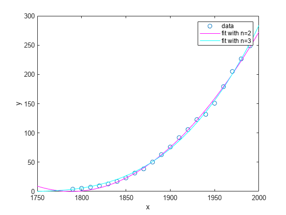
Plot the fit results and the data:
plot(c2,'m')
plot(c3,'c')
legend('data','fit with n=2','fit with n=3')