Arbitrary Magnitude and Phase Filter Design

This example shows how to design filters with customized magnitude and phase specifications. Many filter design problems focus on the magnitude response only, while assuming a linear phase response through symmetry. In some cases, however, the desired filter needs to satisfy constraints on both magnitude and phase.

For example, custom magnitude and phase design specifications can be used for the equalization of magnitude and phase distortions found in data transmission systems (channel equalization) or in oversampled ADC (compensation for non-ideal hardware characteristics). Another application is the design of filters that have smaller group delays than linear phase filters and less distortion than minimum-phase filters for a given order.

Frequency Response Specification and Filter Design

Filter responses are usually specified by frequency intervals (bands) along with the desired gain on each band. Custom magnitude and phase filter specifications are similar, but also include phase response, usually as a complex value encoding both gain and phase response. In most cases, the response specification is comprised of a frequencies vector F = [f1, ..., fN] of N increasing frequencies, and a frequency responses vector H = [h1, ..., hN] corresponding to the filter's complex response values. In DSP System Toolbox™, you can design a filter object with a desired frequency response using the arbmagnphasefir and arbmagnphaseiir responses in designfilt . For more information about FIR and IIR design algorithms, see [1].

FIR Designs

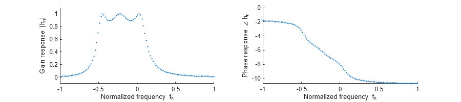
In this first example, we compare several FIR design methods to model the magnitude and phase of a complex RF bandpass filter. First, load the desired filter specification: frequencies to the vector F, and the complex response values to the vector H. Plot the gain and phase frequency responses on the left and the right graphs respectively.

load('gainAndPhase','F','H') % Load frequency response data
plotResponse(F, H) % A helper plotting function used in this demo

Design an arbitrary response FIR filter using the arbmagnphasefir response in designfilt by providing the FilterOrder, Frequencies, and FrequencyResponse arguments. This lets you specify the the desired response on the entire Nyquist range (that is, a single-band specification with no relaxed "don't care" regions). In this example, the desired response data vectors F and H have 655 points, which is relatively dense across the frequency domain.

For a list of supported design methods for each set of input arguments, refer to "argmagnphasefir" filter response in designfilt. When you provide the FilterOrder, Frequencies and FrequencyResponse arguments, the supported design methods are equiripple, ls, and freqsamp. Design the arbitrary response FIR filter using the available methods.

N = 100;
Hd1=designfilt('arbmagnphasefir',Frequencies=F,FrequencyResponse=H,...
    FilterOrder=N,DesignMethod='equiripple',SystemObject=true);
Hd2=designfilt('arbmagnphasefir',Frequencies=F,FrequencyResponse=H,...
    FilterOrder=N,DesignMethod='ls',SystemObject=true);
Hd3=designfilt('arbmagnphasefir',Frequencies=F,FrequencyResponse=H,...
    FilterOrder=N,DesignMethod='freqsamp',SystemObject=true);

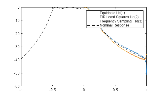
Plot the filters' frequency responses and the nominal response in a dashed line. The equiripple design Hd1 appears to approximate very well on the passband, but slightly deviates in other regions. The least squares design Hd2 is optimized for uniformly weighted quadratic norm (not favoring one region or another), and the frequency sampled FIR design Hd3 appears to exhibit the worst approximation of all three.

figure
[H1,W] = freqz(Hd1);
H2 = freqz(Hd2);
H3 = freqz(Hd3);

plot(W/pi,db(H1))
hold on
plot(W/pi,db(H2))
plot(W/pi,db(H3))
plot(F,db(H),'k--')
hold off
legend('Equiripple Hd(1)', 'FIR Least-Squares Hd(2)','Frequency Sampling  Hd(3)','Nominal Response',Location = 'NorthEast')

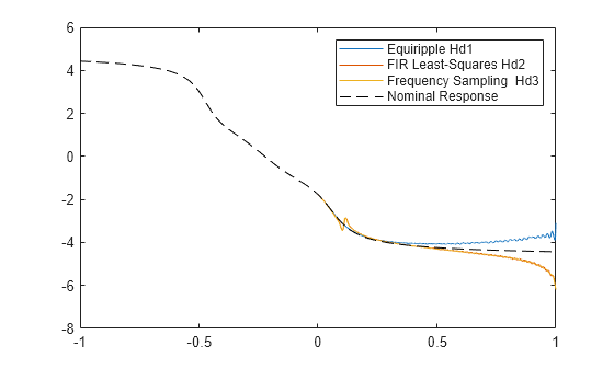
[P1,W] = phasez(Hd1);
P2 = phasez(Hd2);
P3 = phasez(Hd3);

plot(W/pi,P1)
hold on
plot(W/pi,P2)
plot(W/pi,P3)
plot(F,unwrap(angle(H))+2*pi,'k--')
hold off
legend('Equiripple Hd1', 'FIR Least-Squares Hd2','Frequency Sampling  Hd3','Nominal Response')

IIR Designs

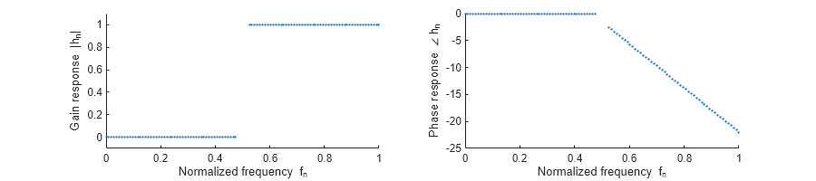
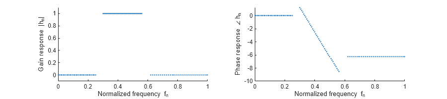
In the next part, we design an IIR filter. The desired filter is a halfband highpass filter with a linear phase on the passband. The specification is given by 100 points on the frequency domain as shown in the following figure.

F = [linspace(0,.475,50) linspace(.525,1,50)];
H = [zeros(1,50) exp(-1j*pi*13*F(51:100))];
plotResponse(F, H)

Create an arbitrary response IIR using argbmagnphaseiir response in designfilt by providing a single-band design specification. This can be done by specifying the NumeratorOrder, DenominatorOrder, Frequencies, and FrequencyResponse arguments. There is only one design method available for this specification - the least squares IIR design (ls).

The ls design method allows to specify different weights for different frequencies, giving more control over the approximation quality of each band. Design the filter with a weight of 1 on the stopband and a weight of 100 on the passband. The high weight given to the passband makes the approximation more accurate on this region.

Nb = 12;
Na = 10;
W = 1*(F<=0.5) + 100*(F>0.5);
Hd = designfilt('arbmagnphaseiir',NumeratorOrder = Nb,DenominatorOrder=Na,Frequencies=F,...
    FrequencyResponse=H, DesignMethod='ls',Weights=W,SystemObject=true);

When using IIR design techniques, the stability of the filter is not guaranteed. Check the IIR stability using the isstable function. To do a more complete analysis, examine the poles and how close they are to the unit circle.

isstable(Hd)

ans = logical
   1

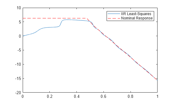
Plot the IIR design response. Note that the approximation on the passband is better than on the stopband, and the phase response is less significant wherever the magnitude gain is small (low dB).

FA = filterAnalyzer(Hd);
setLegendStrings(FA,"IIR Least-Squares")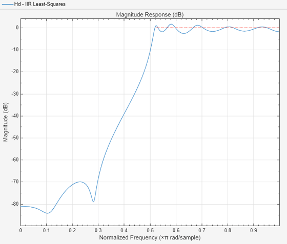

figure
[P,W] = phasez(Hd);
plot(W/pi,P);
hold on
plot(F,unwrap(angle(H))+2*pi,'r--')
hold off
legend('IIR Least-Squares','Nominal Response', Location = 'NorthEast')

Bandpass FIR Design with a Low Group Delay

An interesting application of arbitrary magnitude and phase designs is the design of asymmetric FIR filters that sacrifice linear phase in favor of a shorter group delay. Such filters can still be designed to maintain a good approximation of a linear phase on the passband. Suppose we have three bands for the bandpass filter: a stopband on ${\mathit{F}}_1=[0,0.3)$ and on $$F_3=(0.6,1]$$, and a passband on ${\mathit{F}}_2=\left[0.3,0.6\right]$. On the passband, the desired frequency response is $\mathit{H}\left(\omega \right)={\mathit{e}}^{-\mathit{j}\pi \omega \cdot \mathrm{gd}}$, which has a linear phase response with a group delay of gd.

F1 = linspace(0,.25,30);  % Lower stopband
F2 = linspace(.3,.56,40); % Passband
F3 = linspace(.62,1,30);  % Higher stopband

% Define the desired frequency response on the bands
gd = 12; % Desired Group Delay
P1 = zeros(size(F1));
P2 = exp(-1j*pi*F2*gd);
P3 = zeros(size(F3));
F = [F1 F2 F3];
H = [P1 P2 P3];

Plot the desired frequency response.

plotResponse(F, H)

Create an arbitrary response FIR filter with 3 bands by specifying the FilterOrder = 50, NumBands = 3, followed by 3 pairs of BandFrequencies and BandFrequencyResponse vectors.

N = 50;  % Filter Order
B = 3;   % Number of bands
Hd_mnp = designfilt('arbmagnphasefir',FilterOrder=N,NumBands=B,...
    BandFrequencies1=F1,BandFrequencyResponse1=P1,...
    BandFrequencies2=F2,BandFrequencyResponse2=P2,...
    BandFrequencies3=F3,BandFrequencyResponse3=P3,...
    DesignMethod='equiripple',SystemObject=true);

This design does not have a linear phase, as can be seen by calling the islinphase function.

islinphase(Hd_mnp)

ans = logical
   0

Now, create an arbitrary magnitude filter by only specifying the magnitude response. You can do this using the arbmagfir response in designfilt. Provide the required band frequencies and magnitudes using the pairs of BandFrequencies and BandAmplitudes vectors. The difference between the arbmagnphasefir and arbmagfir responses is that the complex filter response BandFrequencyResponse in arbmagnphasefir is replaced with a magnitude only (nonnegative real) response BandAmplitudes in arbmagfir.

Hd_mo = designfilt('arbmagfir',FilterOrder=N,NumBands=B,...
    BandFrequencies1=F1,BandAmplitudes1=abs(P1),...
    BandFrequencies2=F2,BandAmplitudes2=abs(P2),...
    BandFrequencies3=F3,BandAmplitudes3=abs(P3),...
    DesignMethod='equiripple',SystemObject=true); 

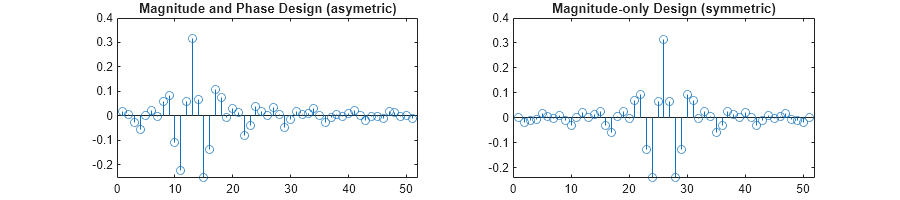
The magnitude-only specification yields symmetric design with a linear phase.

islinphase(Hd_mo)

ans = logical
   1

subplot(1,2,1);
stem(Hd_mnp.Numerator)
title('Magnitude and Phase Design (asymetric)')
subplot(1,2,2);
stem(Hd_mo.Numerator)
title('Magnitude-only Design (symmetric)')

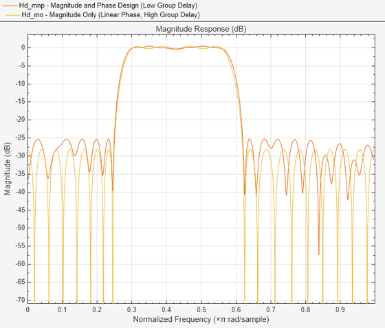
Compare the two designs. Note that they have a very similar bandpass magnitude response.

FA = filterAnalyzer(Hd_mnp, Hd_mo);
setLegendStrings(FA,["Magnitude and Phase Design (Low Group Delay)", ...
    "Magnitude Only (Linear Phase, High Group Delay)"])

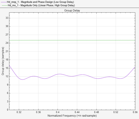
Plot the group delay. The arbitrary magnitude and phase design has a slightly varying group delay. However, the variation is small and on average is 12.5 samples. This group delay is half the group delay of the magnitude only design, which is 25 samples.

FA = filterAnalyzer(Hd_mnp, Hd_mo,Analysis='groupdelay');
setLegendStrings(FA,["Magnitude and Phase Design (Low Group Delay)", ...
    "Magnitude Only (Linear Phase, High Group Delay)"])
zoom(FA,"xy",[0.3 0.56 0 35]);

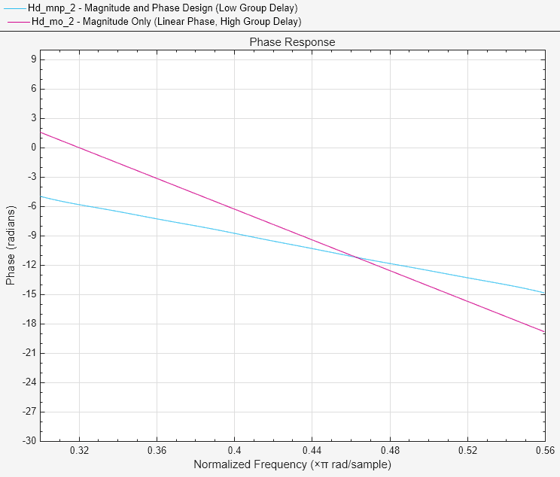
The difference in group delays can also be seen in the phase response. The shallower slope indicates a smaller group delay.

FA = filterAnalyzer(Hd_mnp, Hd_mo,Analysis='phase');
setLegendStrings(FA,["Magnitude and Phase Design (Low Group Delay)", ...
    "Magnitude Only (Linear Phase, High Group Delay)"])
zoom(FA,"xy",[0.3 0.56 -30 10]);

Passband Equalization of a Chebyshev Lowpass Filter

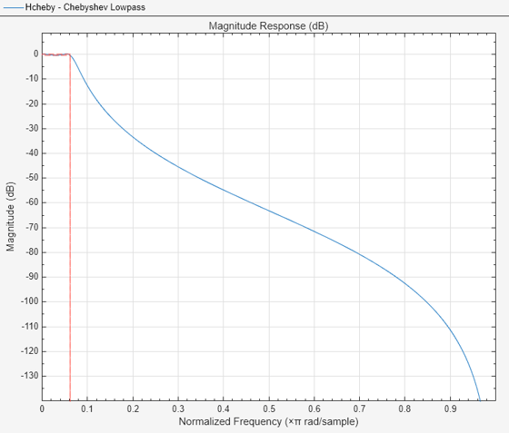
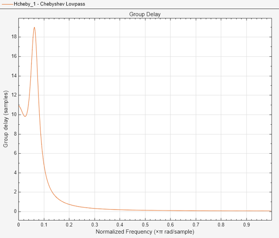
Another common application of arbitrary magnitude-phase designs is the equalization of nonlinear-phase responses of IIR filters. Consider a third order Chebyshev Type I lowpass filter with a normalized passband frequency of 1/16 and passband ripples of 0.5 dB.

Fp = 1/16;  % Passband frequency 
Ap = .5;    % Passband ripples
Hcheby = designfilt('lowpassiir',FilterOrder=3,PassbandFrequency=Fp,...
    PassbandRipple=Ap,DesignMethod='cheby1',SystemObject=true);
FA = filterAnalyzer(Hcheby);
setLegendStrings(FA, 'Chebyshev Lowpass');

Plot the group delay. There is a significant group delay distortion on the passband with group delays ranging from 10 to 20 samples.

FA = filterAnalyzer(Hcheby, Analysis = 'groupdelay');
setLegendStrings(FA,'Chebyshev Lowpass');

To mitigate the distortion in the group delay, an FIR equalizer ${\mathit{H}}_{\mathrm{eq}}\left(\omega \right)$can be used after the IIR filter. Ideally, the combined filter is an ideal lowpass. The combined filter has the passband response $\mathit{G}\left(\omega \right)={\mathit{H}}_{\mathrm{ch}}\left(\omega \right){\mathit{H}}_{\mathrm{eq}}\left(\omega \right)={\mathit{e}}^{-\mathit{j}{\mathit{g}}_{\mathit{d}}\omega }$, eliminating the magnitude ripples to a flat magnitude response and a constant group delay of ${\mathit{g}}_{\mathit{d}}$ samples. The target group ${\mathit{g}}_{\mathit{d}}$ is tied to the allotted FIR length for causal filter designs. In this example, ${\mathit{g}}_{\mathit{d}}=35$ makes a reasonable choice.

To summarize, the equalizer design has two bands:

• On the passband, the desired frequency response of the equalizer should be ${\mathit{H}}_{\mathrm{eq}}\left(\omega \right)={\mathit{e}}^{-\mathit{j}{\mathrm{g}}_{\mathit{d}}\omega }/{\mathit{H}}_{\mathrm{ch}}\left(\omega \right)$.

• On the stopband, the desired response is ${\mathit{H}}_{\mathrm{eq}}\left(\omega \right)=0$, consistent with ${\mathit{H}}_{\mathrm{ch}}$.

This two-band design specification ensures that the FIR approximation of the equalizer focuses on the passband and the stopband only. The remaining parts of the frequency domain are considered don't-care regions.

gd = 35;    % Passband Group Delay of the equalized filter (linear phase)
F1 = 0:5e-4:Fp; % Passband
D1 = exp(-1j*gd*pi*F1)./freqz(Hcheby,F1*pi); 

Fst = 3/16; % Stopband
F2 = linspace(Fst,1,100); 
D2 = zeros(1,length(F2));

There are several FIR design methods that can be used to implement this equalizer FIR specification. Compare the performance using two design methods: a least squares design, and an equiripple design.

Heq_ls = designfilt('arbmagnphasefir',FilterOrder=51,NumBands=2,...
    BandFrequencies1=F1,BandFrequencyResponse1=D1,...
    BandFrequencies2=F2,BandFrequencyResponse2=D2,...
    DesignMethod='ls',SystemObject=true);      % Least-Squares design
Heq_er = designfilt('arbmagnphasefir',FilterOrder=51,NumBands=2,...
    BandFrequencies1=F1,BandFrequencyResponse1=D1,...
    BandFrequencies2=F2,BandFrequencyResponse2=D2,...
    DesignMethod='equiripple',SystemObject=true); % Equiripple design

% Create the cascaded filters
Gls = cascade(Hcheby,Heq_ls);
Geq = cascade(Hcheby,Heq_er);

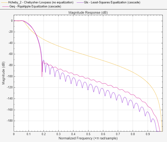
Plot the magnitude responses of the cascaded systems for both filters.

FA = filterAnalyzer(Hcheby,Gls,Geq);
showFilters(FA,false,FilterNames = ["Gls_Stage1","Gls_Stage2","Geq_Stage1","Geq_Stage2"])
setLegendStrings(FA,["Chebyshev Lowpass (no equalization)","Least-Squares Equalization (cascade)", ...
    "Rquiripple Equalization (cascade)"]);

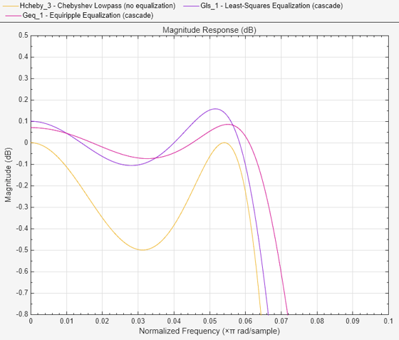
Zoom in around the passband. The passband ripples are attenuated after equalization from 0.5 dB in the original filter to 0.27 dB with the least-squares designed equalizer, and to 0.16 dB with the equiripple designed equalizer.

FA = filterAnalyzer(Hcheby,Gls,Geq);
showFilters(FA,false,FilterNames = ["Gls_1_Stage1","Gls_1_Stage2","Geq_1_Stage1","Geq_1_Stage2"])
setLegendStrings(FA,["Chebyshev Lowpass (no equalization)", ...
    "Least-Squares Equalization (cascade)", ...
    "Equiripple Equalization (cascade)"])
zoom(FA,"xy",[0 .1 -0.8 .5]);

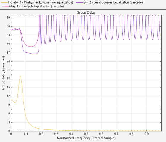
We now turn to the phase (and group delay) equalization. The combined group delay is nearly constant around 35 samples (the target group delay) on the passband. Outside the passband, the combined group delay is seemingly divergent, but this is insignificant as the gain of the filter vanishes on that region.

FA = filterAnalyzer(Hcheby,Gls,Geq,Analysis='groupdelay');
showFilters(FA,false,FilterNames = ["Gls_2_Stage1","Gls_2_Stage2","Geq_2_Stage1","Geq_2_Stage2"])
setLegendStrings(FA,["Chebyshev Lowpass (no equalization)", ...
    "Least-Squares Equalization (cascade)", ...
    "Equiripple Equalization (cascade)"])
zoom(FA,"xy",[0 1 0 40]);

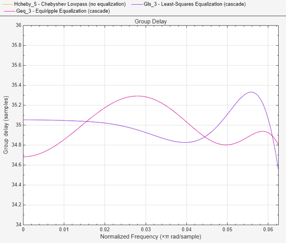
Zoom in around the passband. The group delay in the passband is equalized from a peak-to-peak difference of 8.8 samples to 0.51 samples with the least-squares equalizer, and to 0.62 samples with the equiripple equalizer. Both equalizers perform equally well.

FA = filterAnalyzer(Hcheby,Gls,Geq,Analysis='groupdelay');
showFilters(FA,false,FilterNames = ["Gls_3_Stage1","Gls_3_Stage2","Geq_3_Stage1","Geq_3_Stage2"])
setLegendStrings(FA,["Chebyshev Lowpass (no equalization)", ...
    "Least-Squares Equalization (cascade)", ...
    "Equiripple Equalization (cascade)"])
zoom(FA,"XY",[0 Fp 34 36]);

References

[1] Oppenheim, A.V., and R.W. Schafer, Discrete-Time Signal Processing, Prentice-Hall, 1989.