Frequency-Domain Filtering in HDL

This example shows how to implement a filter in the frequency domain. The filter is built with the FFT and IFFT blocks from DSP HDL Toolbox™.

The model filters sinusoidal input by using the overlap-add method. The overlap-add and the overlap-save filtering methods are area-efficient ways to compute the discrete convolution of a signal with a finite-impulse response (FIR filter). The efficiency gain is significant for high-order filters with a large number of taps. Because of these efficiencies, frequency-domain filtering is a good choice for match filters in communications systems, high-order FIR filters, and channel models on FPGA/ASIC hardware.

Overlap-Add Algorithm

The overlap-add algorithm [1] filters the input signal in the frequency domain. The model divides the input into nonoverlapping blocks and linearly convolves each block with the FIR filter coefficients. To compute the linear convolution of each block, the model multiplies the discrete Fourier transform (DFT) of the block with the filter coefficients, and then finds the inverse DFT of that product. For filter length and FFT size , the model adds the last samples of the linear convolution to the first samples of the next input sequence. The model then returns the first samples of each sum, in sequence.

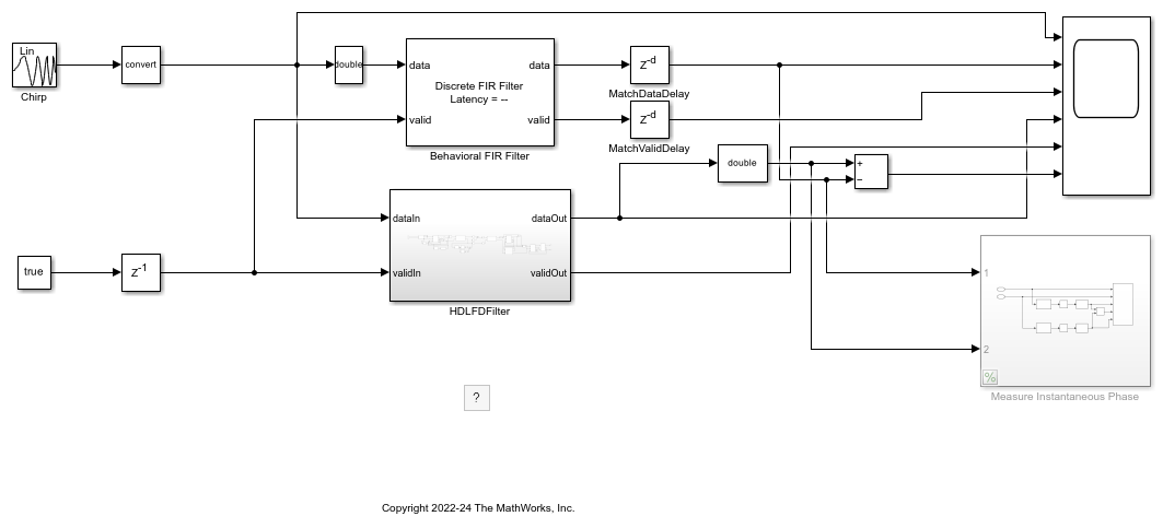
modelname = 'FreqDomainFiltHDL';
open_system(modelname);
set_param(modelname,'SampleTimeColors','on');
set_param(modelname,'Open','on');
set(allchild(0),'Visible','off');

Choosing FFT Size

When selecting an FFT size for a frequency-domain filter, you must make a hardware-friendly choice. If the filter length is an exact power of two, then your FFT size must be exactly double the filter length, . In the case where is a power of two, the filter has no time when it is not adding overlapping results, except for the first input samples. This design simplifies the timing because only the starting period requires special handling.

If the filter length is not an exact power of two, then you must choose an FFT size that is double the next power of two above the filter length, . In this example, the filter has 300 coefficients, so the next power of two is 512. For this case you must choose 1024 for the FFT size. If you use the smaller size of 512, the filter has three types of overlapping regions rather than two, and the hardware design becomes more complicated and area intensive.

Padding and Buffering Samples

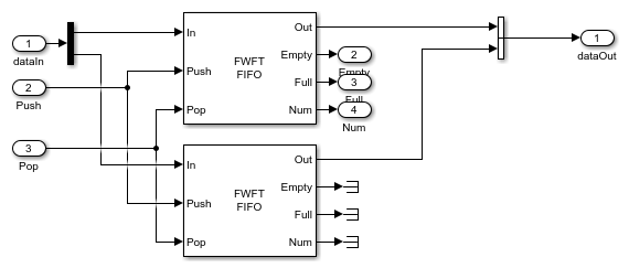
In hardware, computing the FFT of samples requires zero-padding the input to the FFT block at the end of the block of samples. The design must hold the next input samples for the time it takes to pad the block. One way to make up the time is to buffer samples into frames of two samples and process them two per cycle with a frame-based FFT block. The example model uses a FIFO to pair the samples and buffer them until the filter is ready for input.

open_system([modelname '/HDLFDFilter/In FIFO'],'force');

Point Multiplication

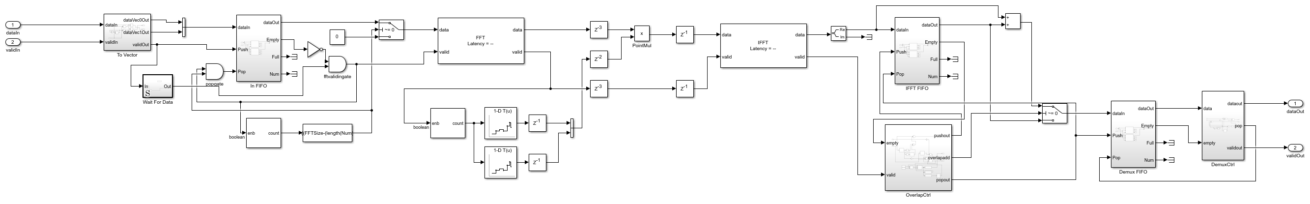
Using a pipelined multipier, the model multiplies the output of the FFT point-by-point with the FFT of the filter coefficients. In this example, the FFT of the filter coefficients is precomputed. If your design used dynamic filter coefficients, you would need another FFT to compute the coefficient transform. An IFFT block then transforms the result of the point multiplication back into the time domain.

open_system([modelname '/HDLFDFilter'],'force');

Design Considerations

Another important consideration in making the frequency-domain filter hardware-friendly is that the shift from one sample at a time to two (or another power of 2) samples at a time means that the point at which the design switches from the nonoverlapped region to the overlapped region must happen on a boundary that is divisible by two (or the selected power of 2) to avoid difficult timing in the design. In other words, the design must switch between the nonoverlapped region and the overlapped region on a boundary that lines up with a complete vector of samples. This requirement adds a condition that your filter length must be divisible by your vector size, which for the 2-sample case means the filter must be an odd-order filter (with an even number of taps).

In this example the filter transfer function is a low-pass filter, so using a chirp or swept tone input signal allows you to easily visualize the frequency response of the filter. For the filter to converge to a solution, you must design it with a larger than default density factor. The filter in this model has 300 taps and is fully symmetric. This filter requires 150 multipliers to implement in the conventional way (time-domain). By using a frequency-domain implementation, you can reduce the multiplier count considerably. When comparing multiplier counts, consider that a time-domain FIR implementation uses real-only multipliers while the FFT, point multiplication, and IFFT in a frequency-domain filter require complex multipliers that use three or four real multipliers each.

Filter Response

You can explore the filter response by looking at the transformed, then quantized, and then inverse-transformed coefficients compared to the original coefficients.

Num is the filter coefficients that you calculated and FFTNum is the transform of those coefficients in double precision. You can simulate the frequency response of the frequency-domain filter by quantizing FFTNum and then transforming that value back into the time domain.

The quantized and transformed filter coefficients for the frequency-domain filter require different quantization settings because they can range between above 1 and below –1. Use Fixed-Point Designer™ to find the best precision binary point for the data by supplying only the signedness and the word length. The fvtool function displayes the data for both the original and the transformed filter coefficients.

QNum = fi(Num,1,18);
QFDNum = ifft(double(fi(FFTNum,1,18)));
QFDNum = QFDNum(1:300);
h = fvtool(double(QNum),1,double(QFDNum),1);
set(h,'OverlayedAnalysis','phase');

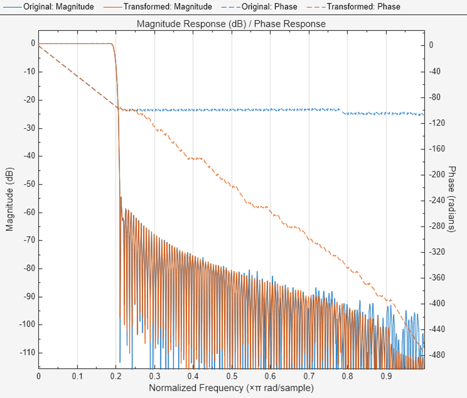
The plot shows the magnitude responses of the two filters match closely with minor variations in the stopband until frequencies near the Nyquist frequency. The phase response matches closely in the passband but varies significantly in the stopband. The original filter shows some ripples but nearly constant phase in the stopband while the frequency-domain filter shows a quantized phase response that falls off rapidly. The phase response of the stopband is not normally a factor in filter design, but it is good to notice that the phase response of the frequency-domain filter does not match the phase response of the original filter.

You can also see the change in stopband phase response by computing the instantaneous phase for both the behavioral FIR filter and the frequency-domain filter. To show this computation, uncomment the Measure Instantaneous Phase subsystem and rerun the simulation. The model computes the instantaneous phase of the real outputs by using the Analytic Signal block, a Complex to Magnitude-Angle block, and finally an Unwrap block to make the phase continuous.

More Design Options

Alternate filter implementation: Another option to implement an HDL frequency-domain filter is the algorithm used in the Frequency-Domain FIR Filter block from the DSP System Toolbox™ library. The block has an option to partition the numerator to reduce latency. When this option is set, the block performs overlap-save or overlap-add on each partition and combines the partial results to form the overall output. The latency is reduced to the partition length. You can use this technique on an HDL frequency-domain filter, but such a filter likely requires more multipliers than the design used in this example.

Alternate ROM implementation: The precomputed transformed filter coefficients are computed from the FFT of a real-valued sequence. This operation produces conjugate symmetric output, which means the upper bins of the FFT are the same values as the lower bins reversed and with the opposite sign on the imaginary part. An alternate design could reduce the size of the ROM used to store the transformed coefficients by half because you can map the upper bins to the lower bins in reverse order and conjugate the result. The first bin, representing the DC value of the sequence, is not included in the repeated values.

Hardware resources: To evaluate your filter design, compare the synthesis results from a time-domain FIR filter with the results from the frequency-domain filter. These results can be hard to predict because they depend on the quantization settings you choose, and because the FFT, point multiplication, and IFFT require complex multipliers that use three or four real multipliers each (depending on block settings). Finding the point where the frequency-domain filter uses less area than the time-domain filter is also challenging. This example model processes vectors of two samples at a time to gain time for the overlap regions and allow continuous input. The vector implementation adds area compared to a scalar implementation. If your application does not require continuous input, then you can acheive a lower-area implementation.

References

[1] Overlap-Add Algorithm: Proakis and Manolakis, Digital Signal Processing, 3rd ed, Prentice-Hall, Englewood Cliffs, NJ, 1996, pp. 430–433.

[2] Overlap-Save Algorithm: Oppenheim and Schafer, Discrete-Time Signal Processing, Prentice-Hall, Englewood Cliffs, NJ, 1989, pp. 558–560.