estimate

Fit univariate regression model with ARIMA errors to data

Syntax

EstMdl = estimate(Mdl,y)

[EstMdl,EstParamCov,logL,info] = estimate(___)

EstMdl = estimate(Mdl,Tbl1)

[EstMdl,EstParamCov,logL,info] = estimate(Mdl,Tbl1)

[___] = estimate(___,Name,Value)

Description

EstMdl = estimate(Mdl,y) returns the fully specified regression model with ARIMA errors EstMdl. This model stores the estimated parameter values resulting from fitting the partially specified, univariate regression model with ARIMA errors Mdl to the observed univariate time series y by using maximum likelihood. EstMdl and Mdl are the same model type and have the same structure.

This syntax specifies an intercept-only regression model.

[EstMdl,EstParamCov,logL,info] = estimate(___) also returns the estimated variance-covariance matrix associated with estimated parameters EstParamCov, the optimized loglikelihood objective function logL, and a data structure of summary information info.

EstMdl = estimate(Mdl,Tbl1) fits the partially specified regression model with ARIMA errors Mdl to response variable and optional predictor data in the input table or timetable Tbl1, which contains time series data, and returns the fully specified, estimated regression model with ARIMA errors EstMdl. estimate selects the response variable named in Mdl.SeriesName or the sole variable in Tbl1. To select a different response variable in Tbl1 to fit the model to, use the ResponseVariable name-value argument. To select predictor variables for the model regression component, use the PredictorVariables name-value argument. (since R2023b)

[EstMdl,EstParamCov,logL,info] = estimate(Mdl,Tbl1) also returns the estimated variance-covariance matrix associated with estimated parameters EstParamCov, the optimized loglikelihood objective function logL, and a data structure of summary information info. (since R2023b)

[___] = estimate(___,Name,Value) specifies options using one or more name-value arguments in addition to any of the input argument combinations in previous syntaxes. estimate returns the output argument combination for the corresponding input arguments. For example, estimate(Mdl,y,U0=u0,X=Pred) fits the regression model with ARIMA errors Mdl to the vector of response data y, specifies the vector of presample regression residual data u0, and includes a linear regression term in the model for the predictor data Pred.

Supply all input data using the same data type. Specifically:

• If you specify the numeric vector y, optional data sets must be numeric arrays and you must use the appropriate name-value argument. For example, to specify a presample, set the Y0 name-value argument to a numeric matrix of presample data.

• If you specify the table or timetable Tbl1, optional data sets must be tables or timetables, respectively, and you must use the appropriate name-value argument. For example, to specify a presample, set the Presample name-value argument to a table or timetable of presample data.

Examples

Compare Model Fits By Using Likelihood Ratio Test

Fit this regression model with ARMA(2,1) errors to simulated data:

$$\begin{array}{l}\begin{array}{c}{y}_t=1+X_t\left[\begin{array}{c}0.1\\ -0.2\end{array}\right]+u_t\\ u_t=0.5u_{t-1}-0.8u_{t-2}+{\epsilon }_t-0.5{\epsilon }_{t-1},\end{array}\end{array}$$

where $${\epsilon }_t$$ is Gaussian with variance 0.1. Compare the fit to an intercept-only regression model by conducting a likelihood ratio test. Provide response and predictor data in vectors.

Simulate Data

Specify the regression model with ARMA(2,1) errors. Simulate responses from the model, and simulate two predictor series from the standard Gaussian distribution.

Mdl0 = regARIMA(Intercept=1,AR={0.5 -0.8},MA=-0.5, ...
    Beta=[0.1; -0.2],Variance=0.1);

rng(1,"twister")  % For reproducibility
Pred =  randn(100,2);
y = simulate(Mdl0,100,X=Pred);

y is a 100-by-1 random response path simulated from Mdl0.

Fit Unrestricted Model

Create an unrestricted model template of a regression model with ARMA(2,1) errors for estimation.

Mdl = regARIMA(2,0,1)

Mdl = 
  regARIMA with properties:

     Description: "ARMA(2,1) Error Model (Gaussian Distribution)"
      SeriesName: "Y"
    Distribution: Name = "Gaussian"
       Intercept: NaN
            Beta: [1×0]
               P: 2
               Q: 1
              AR: {NaN NaN} at lags [1 2]
             SAR: {}
              MA: {NaN} at lag [1]
             SMA: {}
        Variance: NaN

The AR coefficients, MA coefficients, and the innovation variance are NaN values. estimate estimates those parameters. When Beta is an empty array, estimate determines the number of regression coefficients to estimate.

Fit the unrestricted model to the data. Specify the predictor data. Return the optimized loglikelihood.

[EstMdlUR,~,logLUR] = estimate(Mdl,y,X=Pred);

 
    Regression with ARMA(2,1) Error Model (Gaussian Distribution):
 
                  Value      StandardError    TStatistic      PValue  
                 ________    _____________    __________    __________

    Intercept      1.0167      0.010154         100.13               0
    AR{1}         0.64995      0.093794         6.9295      4.2226e-12
    AR{2}        -0.69174      0.082575        -8.3771      5.4247e-17
    MA{1}        -0.64508       0.11055         -5.835      5.3796e-09
    Beta(1)       0.10866      0.020965          5.183      2.1835e-07
    Beta(2)      -0.20979      0.022824        -9.1917      3.8679e-20
    Variance     0.073117      0.008716         8.3888      4.9121e-17

EstMdlUR is a fully specified regARIMA object representing the estimated unrestricted regression model with ARIMA errors.

Fit Restricted Model

The restricted model contains the same error model, but the regression model contains only an intercept. That is, the restricted model imposes two restrictions on the unrestricted model: ${\beta }_1={\beta }_2=0$.

Fit the restricted model to the data. Return the optimized loglikelihood.

[EstMdlR,~,logLR] = estimate(Mdl,y);

 
    ARMA(2,1) Error Model (Gaussian Distribution):
 
                  Value      StandardError    TStatistic      PValue  
                 ________    _____________    __________    __________

    Intercept      1.0176      0.024905         40.859               0
    AR{1}         0.51541       0.18536         2.7805       0.0054271
    AR{2}        -0.53359       0.10949        -4.8735      1.0963e-06
    MA{1}        -0.34923       0.19423         -1.798         0.07218
    Variance       0.1445      0.020214         7.1486      8.7671e-13

EstMdlR is a fully specified regARIMA object representing the estimated restricted regression model with ARIMA errors.

Conduct Likelihood Ratio Test

The likelihood ratio test requires the optimized loglikelihoods of the unrestricted and restricted models, and it requires the number of model restrictions (degrees of freedom).

Conduct a likelihood ratio test to determine which model has the better fit to the data.

dof = 2;
[h,p] = lratiotest(logLUR,logLR,dof)

h = logical
   1

p = 
1.6653e-15

The $\mathit{p}$-value is close to zero, which suggests that there is strong evidence to reject the null hypothesis that the data fits the restricted model better than the unrestricted model.

Fit Regression Model With ARIMA Errors to Response and Predictor Variables in Timetable

Since R2023b

Fit a regression model with ARMA(1,1) errors by regressing the US consumer price index (CPI) quarterly changes onto the US gross domestic product (GDP) growth rate. Supply a timetable of data and specify the series for the fit.

Load and Transform Data

Load the US macroeconomic data set. Compute the series of GDP quarterly growth rates and CPI quarterly changes.

load Data_USEconModel
DTT = price2ret(DataTimeTable,DataVariables="GDP");
DTT.GDPRate = 100*DTT.GDP;
DTT.CPIDel = diff(DataTimeTable.CPIAUCSL);
T = height(DTT) 

T = 
248

figure
tiledlayout(2,1)
nexttile
plot(DTT.Time,DTT.GDPRate)
title("GDP Rate")
ylabel("Percent Growth")
nexttile
plot(DTT.Time,DTT.CPIDel)
title("Index")

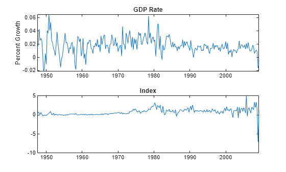
The series appear stationary, albeit heteroscedastic.

Prepare Timetable for Estimation

When you plan to supply a timetable, you must ensure it has all the following characteristics:

• The selected response variable is numeric and does not contain any missing values.

• The timestamps in the Time variable are regular, and they are ascending or descending.

Remove all missing values from the timetable.

DTT = rmmissing(DTT);
T_DTT = height(DTT)

T_DTT = 
248

Because each sample time has an observation for all variables, rmmissing does not remove any observations.

Determine whether the sampling timestamps have a regular frequency and are sorted.

areTimestampsRegular = isregular(DTT,"quarters")

areTimestampsRegular = logical
   0

areTimestampsSorted = issorted(DTT.Time)

areTimestampsSorted = logical
   1

areTimestampsRegular = 0 indicates that the timestamps of DTT are irregular. areTimestampsSorted = 1 indicates that the timestamps are sorted. Macroeconomic series in this example are timestamped at the end of the month. This quality induces an irregularly measured series.

Remedy the time irregularity by shifting all dates to the first day of the quarter.

dt = DTT.Time;
dt = dateshift(dt,"start","quarter");
DTT.Time = dt;
areTimestampsRegular = isregular(DTT,"quarters")

areTimestampsRegular = logical
   1

DTT is regular.

Create Model Template for Estimation

Suppose that a regression model of CPI quarterly changes onto the GDP rate, with ARMA(1,1) errors, is appropriate.

Create a model template for a regression model with ARMA(1,1) errors template.

Mdl = regARIMA(1,0,1)

Mdl = 
  regARIMA with properties:

     Description: "ARMA(1,1) Error Model (Gaussian Distribution)"
      SeriesName: "Y"
    Distribution: Name = "Gaussian"
       Intercept: NaN
            Beta: [1×0]
               P: 1
               Q: 1
              AR: {NaN} at lag [1]
             SAR: {}
              MA: {NaN} at lag [1]
             SMA: {}
        Variance: NaN

Mdl is a partially specified regARIMA object.

Fit Model to Data

Fit a regression model with ARMA(1,1) errors to the data. Specify the entire series GDP rate and CPI quarterly changes series, and specify the response and predictor variable names.

EstMdl = estimate(Mdl,DTT,ResponseVariable="GDPRate", ...
    PredictorVariables="CPIDel");

 
    Regression with ARMA(1,1) Error Model (Gaussian Distribution):
 
                  Value      StandardError    TStatistic      PValue  
                 ________    _____________    __________    __________

    Intercept      0.0162      0.0016077        10.077      6.9994e-24
    AR{1}         0.60515       0.089912        6.7305      1.6906e-11
    MA{1}        -0.16221        0.11051       -1.4678         0.14216
    Beta(1)      0.002221     0.00077691        2.8587       0.0042532
    Variance     0.000113     7.2753e-06        15.533      2.0838e-54

EstMdl is a fully specified, estimated regARIMA object. By default, estimate backcasts for the required Mdl.P = 1 presample regression model residual and sets the required Mdl.Q = 1 presample error model residual to 0.

Initialize Model By Providing Pilot Sample Estimates

Since R2023b

Fit a regression model with ARMA(1,1) errors by regressing the US CPI quarterly changes onto the US GDP growth rate. Obtain initial parameter values by fitting a pilot sample.

Load the US macroeconomic data set. Compute the series of GDP quarterly growth rates and CPI quarterly changes.

load Data_USEconModel
DTT = price2ret(DataTimeTable,DataVariables="GDP");
DTT.GDPRate = 100*DTT.GDP;
DTT.CPIDel = diff(DataTimeTable.CPIAUCSL);
T = height(DTT); % Effective sample size

Remedy the time irregularity by shifting all dates to the first day of the quarter.

dt = DTT.Time;
dt = dateshift(dt,"start","quarter");
DTT.Time = dt;

Suppose that a regression model of CPI quarterly changes onto the GDP rate, with ARMA(1,1) errors, is appropriate.

Create a model template for a regression model with ARMA(1,1) errors template. Specify the response series name as GDPRate.

Mdl = regARIMA(1,0,1);
Mdl.SeriesName = "GDPRate";

Fit the model to a pilot sample of approximately the first 25% of the data. Defer to default initial parameter values.

cutoff = floor(0.25*T);

DTT0 = DTT(1:cutoff,:);
DTT1 = DTT((cutoff+1):end,:);
EstMdl0 = estimate(Mdl,DTT0,PredictorVariables="CPIDel"); 

 
    Regression with ARMA(1,1) Error Model (Gaussian Distribution):
 
                   Value       StandardError    TStatistic      PValue  
                 __________    _____________    __________    __________

    Intercept      0.012032      0.0041096        2.9279       0.0034126
    AR{1}           0.35741        0.31565        1.1323         0.25751
    MA{1}          0.059366        0.32435       0.18303         0.85477
    Beta(1)        0.029888       0.011311        2.6423       0.0082335
    Variance     0.00020617     3.9244e-05        5.2535      1.4921e-07

EstMdl0 is a regression model with ARMA(1,1) errors fit to the pilot sample. It contains parameter estimates, with which to initialize the model to fit to the remaining 75% of the data set.

Fit the model to the remaining data. Initialize the optimization algorithm by specifying the parameter estimates obtained from fitting the model to the pilot sample. Also, provide presample regression and error model residuals from the pilot sample fit.

intercept0 = EstMdl0.Intercept;
ar0        = EstMdl0.AR{1};
ma0        = EstMdl0.MA{1};
variance0  = EstMdl0.Variance;
beta0      = EstMdl0.Beta;

PresampleTbl = infer(EstMdl0,DTT0,ResponseVariable="GDPRate", ...
    PredictorVariables="CPIDel"); % Presample residuals

EstMdl1 = estimate(Mdl,DTT1,PredictorVariables="CPIDel",Presample=PresampleTbl, ...
    PresampleInnovationVariable="GDPRate_ErrorResidual", ...
    PresampleRegressionDisturbanceVariable="GDPRate_RegressionResidual", ...
    Intercept0=intercept0,AR0=ar0,MA0=ma0,Variance0=variance0,Beta0=beta0);

 
    Regression with ARMA(1,1) Error Model (Gaussian Distribution):
 
                   Value       StandardError    TStatistic     PValue  
                 __________    _____________    __________    _________

    Intercept      0.015837      0.0044514        3.5578       0.000374
    AR{1}           0.97895       0.022658        43.205              0
    MA{1}          -0.83051       0.049504       -16.777      3.616e-63
    Beta(1)       0.0023693     0.00077788        3.0458      0.0023204
    Variance     7.6585e-05     5.6687e-06         13.51      1.362e-41

Input Arguments

Mdl — Partially specified regression model with ARIMA errors

regARIMA model object

Partially specified regression model with ARIMA errors, used to indicate constrained and estimable model parameters, specified as an regARIMA model object returned by regARIMA. Properties of Mdl describe the model structure and can specify parameter values.

estimate fits unspecified (NaN-valued) parameters to the data y.

estimate treats specified parameters as equality constraints during estimation.

y — Single path of observed response data y_t

numeric column vector

Single path of observed response data y_t, to which the model Mdl is fit, specified as a numobs-by-1 numeric column vector. The last observation of y is the latest observation.

Data Types: double

Tbl1 — Time series data

table | timetable

Since R2023b

Time series data, to which estimate fits the model, specified as a table or timetable with numvars variables and numobs rows.

The selected response variable is a numeric vector representing a single path of numobs observations. You can optionally select a response variable y_t from Tbl1 by using the ResponseVariables name-value argument, and you can select numpreds predictor variables x_t for the linear regression component by using the PredictorVariables name-value argument.

Each row is an observation, and measurements in each row occur simultaneously. Variables in Tbl1 represent the continuation of corresponding variables in Presample.

If Tbl1 is a timetable, it must represent a sample with a regular datetime time step (see isregular), and the datetime vector Tbl1.Time must be strictly ascending or descending.

If Tbl1 is a table, the last row contains the latest observation.

Name-Value Arguments

Specify optional pairs of arguments as Name1=Value1,...,NameN=ValueN, where Name is the argument name and Value is the corresponding value. Name-value arguments must appear after other arguments, but the order of the pairs does not matter.

Before R2021a, use commas to separate each name and value, and enclose Name in quotes.

Example: esimtate(Mdl,y,U0=u0,X=Pred) uses the vector u0 as presample regression residual data to initialize the error model for estimation, and includes a linear regression component for the predictor data in the vector Pred.

Estimation Options

ResponseVariable — Response variable y_t to select from Tbl1

string scalar | character vector | integer | logical vector

Since R2023b

Response variable y_t to select from Tbl1 containing the response data, specified as one of the following data types:

• String scalar or character vector containing a variable name in Tbl1.Properties.VariableNames

• Variable index (integer) to select from Tbl1.Properties.VariableNames

• A length numvars logical vector, where ResponseVariable(j) = true selects variable j from Tbl1.Properties.VariableNames, and sum(ResponseVariable) is 1

The selected variable must be a numeric vector and cannot contain missing values (NaN).

If Tbl1 has one variable, the default specifies that variable. Otherwise, the default matches the variable to name in Mdl.SeriesName.

Example: ResponseVariable="StockRate2"

Example: ResponseVariable=[false false true false] or ResponseVariable=3 selects the third table variable as the response variable.

Data Types: double | logical | char | cell | string

X — Predictor data

numeric matrix

Predictor data for the linear regression component, specified as a numeric matrix containing numpreds columns. Use X only when you supply a vector of response data y.

numpreds is the number of predictor variables.

Rows correspond to observations, and the last row contains the latest observation. estimate does not use the regression component in the presample period. X must have at least numobs observations. If you supply more rows than necessary, estimate uses the latest observations only. estimate synchronizes X and y so that the latest observations (last rows) occur simultaneously.

Columns correspond to individual predictor variables.

By default, estimate excludes the regression component, regardless of its presence in Mdl.

Data Types: double

PredictorVariables — Predictor variables x_t to select from Tbl1

string vector | cell vector of character vectors | vector of integers | logical vector

Since R2023b

Predictor variables x_t to select from Tbl1 containing predictor data for the regression component, specified as one of the following data types:

• String vector or cell vector of character vectors containing numpreds variable names in Tbl1.Properties.VariableNames

• A length numpreds vector of unique indices (positive integers) of variables to select from Tbl1.Properties.VariableNames

• A length numvars logical vector, where PredictorVariables(j) = true selects variable j from Tbl1.Properties.VariableNames

The selected variables must be numeric vectors and cannot contain missing values (NaN).

By default, estimate excludes the regression component, regardless of its presence in Mdl.

Example: PredictorVariables=["M1SL" "TB3MS" "UNRATE"]

Example: PredictorVariables=[true false true false] or PredictorVariable=[1 3] selects the first and third table variables to supply the predictor data.

Data Types: double | logical | char | cell | string

Options — Optimization options

optimoptions optimization controller

Optimization options, specified as an optimoptions optimization controller. For details on modifying the default values of the optimizer, see optimoptions or fmincon in Optimization Toolbox™.

For example, to change the constraint tolerance to 1e-6, set options = optimoptions(@fmincon,ConstraintTolerance=1e-6,Algorithm="sqp"). Then, pass Options into estimate using Options=options.

By default, estimate uses the same default options as fmincon, except Algorithm is "sqp" and ConstraintTolerance is 1e-7.

Display — Command Window display option

"params" (default) | "diagnostics" | "full'" | "iter" | "off" | string vector | cell vector of character vectors

Command Window display option, specified as one or more of the values in this table.

Value	Information Displayed
"diagnostics"	Optimization diagnostics
"full"	Maximum likelihood parameter estimates, standard errors, t statistics, iterative optimization information, and optimization diagnostics
"iter"	Iterative optimization information
"off"	None
"params"	Maximum likelihood parameter estimates, standard errors, and t statistics and p-values of coefficient significance tests

Example: Display="off" is well suited for running a simulation that estimates many models.

Example: Display=["params" "diagnostics"] displays all estimation results and the optimization diagnostics.

Data Types: char | cell | string

Presample Specifications

E0 — Presample error model residual data associated with model innovations ε_t

numeric column vector

Presample error model residual data associated with the model innovations ε_t, specified as a numpreobs-by-1 numeric column vector. E0 initializes the error model moving average (MA) component. estimate assumes E0 has a mean of 0. Use E0 only when you supply the vector of response data y.

numpreobs is the number of presample observations. Each row is a presample observation. The last row contains the latest presample observation. numpreobs must be at least Mdl.Q. If numpreobs > Mdl.Q, estimate uses the latest required number of observations only. The last element or row contains the latest observation.

By default, estimate sets all required presample error model residuals to 0, which is the expected value of the corresponding innovations series.

Data Types: double

U0 — Presample regression residual data associated with unconditional disturbances u_t

numeric column vector

Presample regression residual data associated with the unconditional disturbances u_t, specified as a numpreobs-by-1 numeric column vector. U0 initializes the error model autoregressive (AR) component. Use U0 only when you supply the vector of response data y.

numpreobs is the number of presample observations. Each row is a presample observation. The last row contains the latest presample observation. numpreobs must be at least Mdl.P. If numpreobs > Mdl.P, estimate uses the latest required number of observations only. The last element or row contains the latest observation.

By default, estimate backcasts the error model for the required presample unconditional disturbances.

Data Types: double

Presample — Presample data

table | timetable

Since R2023b

Presample data containing the error model residual series, associated with the model innovations ε_t, or the regression residual series, associated with the unconditional disturbances u_t, to initialize the model for estimation, specified as a table or timetable, the same type as Tbl1, with numprevars variables and numpreobs rows. Use Presample only when you supply a table or timetable of data Tbl1.

Each selected variable is a single path of numpreobs observations representing the presample of error or regression model residuals associated the selected response variable in Tbl1.

Each row is a presample observation, and measurements in each row occur simultaneously. numpreobs must satisfy one of the following conditions:

• numpreobs ≥ Mdl.P when Presample provides only presample regression model residuals

• numpreobs ≥ Mdl.Q when Presample provides only presample error model residuals

• numpreobs ≥ max([Mdl.P Mdl.Q]) when Presample provides presample error and regression model residuals.

If you supply more rows than necessary, estimate uses the latest required number of observations only.

If Presample is a timetable, all the following conditions must be true:

• Presample must represent a sample with a regular datetime time step (see isregular).

• The inputs Tbl1 and Presample must be consistent in time such that Presample immediately precedes Tbl1 with respect to the sampling frequency and order.

• The datetime vector of sample timestamps Presample.Time must be ascending or descending.

If Presample is a table, the last row contains the latest presample observation.

By default, estimate backcasts for necessary presample regression model residuals and it sets necessary presample error model residuals to zero.

If you specify Presample, you must specify at least one of the presample regression or error model residual variable names by using the PresampleRegressionDisturbanceVariable or PresampleInnovationVariable name-value argument, respectively.

PresampleInnovationVariable — Error model residual variable to select from Presample

string scalar | character vector | integer | logical vector

Since R2023b

Error model residual variable to select from Presample containing presample error model residual data, associated with the model innovations ε_t, specified as one of the following data types:

• String scalar or character vector containing the variable name to select from Presample.Properties.VariableNames

• Variable index (positive integer) to select from Presample.Properties.VariableNames

• A logical vector, where PresampleInnovationVariable(j) = true selects variable j from Presample.Properties.VariableNames

The selected variable must be a numeric vector and cannot contain missing values (NaNs).

If you specify presample error model residual data by using the Presample name-value argument, you must specify PresampleInnovationVariable.

Example: PresampleInnovationVariable="GDPInnov"

Example: PresampleInnovationVariable=[false false true false] or PresampleInnovationVariable=3 selects the third table variable for presample error model residual data.

Data Types: double | logical | char | cell | string

PresampleRegressionDistrubanceVariable — Regression model residual variable to select from Presample

string scalar | character vector | integer | logical vector

Since R2023b

Regression model residual variable to select from Presample containing presample data for the regression model residuals, associated with the unconditional disturbances u_t, specified as one of the following data types:

• String scalar or character vector containing a variable name in Presample.Properties.VariableNames

• Variable index (positive integer) to select from Presample.Properties.VariableNames

• A logical vector, where PresampleRegressionDistrubanceVariable(j) = true selects variable j from Presample.Properties.VariableNames

The selected variable must be a numeric vector and cannot contain missing values (NaNs).

If you specify presample regression residual data by using the Presample name-value argument, you must specify PresampleRegressionDistrubanceVariable.

Example: PresampleRegressionDistrubanceVariable="StockRateU"

Example: PresampleRegressionDistrubanceVariable=[false false true false] or PresampleRegressionDistrubanceVariable=3 selects the third table variable as the presample regression model residual data.

Data Types: double | logical | char | cell | string

Initial Parameter Value Specifications

Intercept0 — Initial estimate of regression model intercept c

numeric scalar

Initial estimate of the regression model intercept c, specified as a numeric scalar.

By default, estimate derives initial estimates using standard time series techniques.

Data Types: double

AR0 — Initial estimates of nonseasonal autoregressive (AR) polynomial coefficients ɑ(L)

numeric vector

Initial estimates of the nonseasonal AR polynomial coefficients ɑ(L), specified as a numeric vector.

Elements of AR0 correspond to nonzero cells of Mdl.AR.

By default, estimate derives initial estimates using standard time series techniques.

Data Types: double

SAR0 — Initial estimates of seasonal AR polynomial coefficients A(L)

numeric vector

Initial estimates of the seasonal AR polynomial coefficients A(L), specified as a numeric vector.

Elements of SAR0 correspond to nonzero cells of Mdl.SAR.

By default, estimate derives initial estimates using standard time series techniques.

Data Types: double

MA0 — Initial estimates of nonseasonal moving average (MA) polynomial coefficients b(L)

numeric vector

Initial estimates of the nonseasonal MA polynomial coefficients b(L), specified as a numeric vector.

Elements of MA0 correspond to elements of Mdl.MA.

By default, estimate derives initial estimates using standard time series techniques.

Data Types: double

SMA0 — Initial estimates of seasonal MA polynomial coefficients B(L)

numeric vector

Initial estimates of the seasonal moving average polynomial coefficients B(L), specified as a numeric vector.

Elements of SMA0 correspond to nonzero cells of Mdl.SMA.

By default, estimate derives initial estimates using standard time series techniques.

Data Types: double

Beta0 — Initial estimates of regression coefficients

numeric vector

Initial estimates of the regression coefficients β, specified as a numeric vector.

The length of Beta0 must equal the numpreds. Elements of Beta0 correspond to the predictor variables represented by the columns of X or PredictorVariables.

By default, estimate derives initial estimates using standard time series techniques.

Data Types: double

DoF0 — Initial estimate of t-distribution degrees-of-freedom parameter

10 (default) | positive scalar

Initial estimate of the t-distribution degrees-of-freedom parameter ν, specified as a positive scalar. DoF0 must exceed 2.

Data Types: double

Variance0 — Initial estimates of error model innovation variance σ_t²

positive scalar

Initial estimate of the error model innovation variance σ_t², specified as a positive scalar.

By default, estimate derives initial estimates using standard time series techniques.

Example: Variance0=2

Data Types: double

Note

• NaN values in y, X, E0, and U0 indicate missing values. estimate removes missing values from specified data by listwise deletion.

  • For the presample, estimate horizontally concatenates E0 and U0, and then it removes any row of the concatenated matrix containing at least one NaN.

  • For the estimation sample, estimate horizontally concatenates y and X, and then it removes any row of the concatenated matrix containing at least one NaN.

  • Regardless of sample, estimate synchronizes the specified, possibly jagged vectors with respect to the latest observation of the sample (last row).

  This type of data reduction reduces the effective sample size and can create an irregular time series.

• estimate issues an error when any table or timetable input contains missing values.

• The intercept c of a regression model with ARIMA errors having nonzero degrees of seasonal or nonseasonal integration, Mdl.Seasonality or Mdl.D, is not identifiable. In other words, estimate cannot estimate an intercept of a regression model with ARIMA errors that has nonzero degrees of seasonal or nonseasonal integration. If you pass in such a model for estimation, estimate displays a warning in the Command Window and sets EstMdl.Intercept to NaN.

• If you specify the Display name-value argument, the value takes precedence over the specifications of the optimization options Diagnostics and Display. Otherwise, estimate honors all selections related to the display of optimization information in the optimization options.

Output Arguments

EstMdl — Estimated regression model with ARIMA errors

regARIMA model object

Estimated regression model with ARIMA errors, returned as a regARIMA model object. estimate uses maximum likelihood to calculate all parameter estimates not constrained by Mdl (that is, it estimates all parameters in Mdl that you set to NaN).

EstMdl is a copy of Mdl that has NaN values replaced with parameter estimates. EstMdl is fully specified.

EstParamCov — Estimated covariance matrix of maximum likelihood estimates

positive semidefinite numeric matrix

Estimated covariance matrix of maximum likelihood estimates known to the optimizer, returned as a positive semidefinite numeric matrix.

The rows and columns contain the covariances of the parameter estimates. The standard error of each parameter estimate is the square root of the main diagonal entries.

The rows and columns corresponding to any parameters held fixed as equality constraints are zero vectors.

Parameters corresponding to the rows and columns of EstParamCov appear in the following order:

• Intercept

• Nonzero AR coefficients at positive lags, from the smallest to largest lag

• Nonzero SAR coefficients at positive lags, from the smallest to largest lag

• Nonzero MA coefficients at positive lags, from the smallest to largest lag

• Nonzero SMA coefficients at positive lags, from the smallest to largest lag

• Regression coefficients (when you specify exogenous data), ordered by the columns of X or entries of PredictorVariables

• Innovations variance

• Degrees of freedom (t-innovation distribution only)

estimate uses the outer product of gradients (OPG) method to perform covariance matrix estimation.

Data Types: double

logL — Optimized loglikelihood objective function value

numeric scalar

Optimized loglikelihood objective function value, returned as a numeric scalar.

Data Types: double

info — Optimization summary

structure array

Optimization summary, returned as a structure array with the fields described in this table.

Field	Description
exitflag	Optimization exit flag (see fmincon in Optimization Toolbox)
options	Optimization options controller (see optimoptions and fmincon in Optimization Toolbox)
X	Vector of final parameter estimates
X0	Vector of initial parameter estimates

For example, you can display the vector of final estimates by entering info.X in the Command Window.

Data Types: struct

Tips

• To access values of the estimation results, including the number of free parameters in the model, pass EstMdl to summarize.

Algorithms

estimate estimates the parameters as follows:

1. Initialize the model by applying initial data and parameter values.

2. Infer the unconditional disturbances from the regression model.

3. Infer the residuals of the ARIMA error model.

4. Use the distribution of the innovations to build the likelihood function.

5. Maximize the loglikelihood function with respect to the parameters using fmincon.

References

[1] Box, George E. P., Gwilym M. Jenkins, and Gregory C. Reinsel. Time Series Analysis: Forecasting and Control. 3rd ed. Englewood Cliffs, NJ: Prentice Hall, 1994.

[2] Davidson, R., and J. G. MacKinnon. Econometric Theory and Methods. Oxford, UK: Oxford University Press, 2004.

[3] Enders, Walter. Applied Econometric Time Series. Hoboken, NJ: John Wiley & Sons, Inc., 1995.

[4] Hamilton, James D. Time Series Analysis. Princeton, NJ: Princeton University Press, 1994.

[5] Pankratz, A. Forecasting with Dynamic Regression Models. John Wiley & Sons, Inc., 1991.

[6] Tsay, R. S. Analysis of Financial Time Series. 2nd ed. Hoboken, NJ: John Wiley & Sons, Inc., 2005.

Version History

Introduced in R2013b

R2023b: estimate accepts input data in tables and timetables

In addition to accepting input data (in-sample and presample data) in numeric arrays, estimate accepts input data in tables or regular timetables. When you supply data in a table or timetable, estimate chooses the default series on which to operate, but you can use the specified optional name-value argument to select a different series.

Name-value arguments to support tabular workflows include:

• ResponseVariable specifies the variable name of the response series in the input data Tbl1, to which the model is fit.

• PredictorVariables specifies the names of the predictor series to select from the input data for the model regression component.

• Presample specifies the input table or timetable of presample response, regression model residual, and error model residual data.

• PresampleResponseVariable specifies the variable name of the response series to select from Presample.

• PresampleInnovationVariable specifies the variable name of the error model residual series to select from Presample.

• PresampleRegressionDisturbanceVariable specifies the name of the regression residual series to select from Presample.

R2019b: estimate includes the final lag in all estimated univariate time series model polynomials

estimate includes the final polynomial lag as specified in the input model template for estimation. In other words, the specified polynomial degrees of an input model template returned by an object creation function and the corresponding polynomial degrees of the estimated model returned by estimate are equal.

Before R2019b, estimate removed trailing lags estimated below the tolerance of 1e-12.

Update Code

Polynomial degrees require minimum presample observations for operations downstream of estimation, such as model forecasting and simulation. If a model template in your code does not describe the data generating process well, then the polynomials in the estimated model can have higher degrees than in previous releases. Consequently, you must supply additional presample responses for operations on the estimated model; otherwise, the function issues an error. For more details, see the Y0 name-value argument.