Time Series Regression I: Linear Models
This example introduces basic assumptions behind multiple linear regression models. It is the first in a series of examples on time series regression, providing the basis for all subsequent examples.
Multiple Linear Models
Time series processes are often described by multiple linear regression (MLR) models of the form:
where is an observed response and includes columns for contemporaneous values of observable predictors. The partial regression coefficients in represent the marginal contributions of individual predictors to the variation in when all of the other predictors are held fixed.
The term is a catch-all for differences between predicted and observed values of . These differences are due to process fluctuations (changes in ), measurement errors (changes in ), and model misspecifications (for example, omitted predictors or nonlinear relationships between and ). They also arise from inherent stochasticity in the underlying data-generating process (DGP), which the model attempts to represent. It is usually assumed that is generated by an unobservable innovations process with stationary covariance
for any time interval of length . Under some further basic assumptions about , , and their relationship, reliable estimates of are obtained by ordinary least squares (OLS).
As in other social sciences, economic data are usually collected by passive observation, without the aid of controlled experiments. Theoretically relevant predictors may need to be replaced by practically available proxies. Economic observations, in turn, may have limited frequency, low variability, and strong interdependencies.
These data shortcomings lead to a number of issues with the reliability of OLS estimates and the standard statistical techniques applied to model specification. Coefficient estimates may be sensitive to data measurement errors, making significance tests unreliable. Simultaneous changes in multiple predictors may produce interactions that are difficult to separate into individual effects. Observed changes in the response may be correlated with, but not caused by, observed changes in the predictors.
Assessing model assumptions in the context of available data is the goal of specification analysis. When the reliability of a model becomes suspect, practical solutions may be limited, but a thorough analysis can help to identify the source and degree of any problems.
This is the first in a series of examples that discuss basic techniques for specifying and diagnosing MLR models. The series also offers some general strategies for addressing the specific issues that arise when working with economic time series data.
Classical Assumptions
Classical linear model (CLM) assumptions allow OLS to produce estimates with desirable properties [3]. The fundamental assumption is that the MLR model, and the predictors selected, correctly specify a linear relationship in the underlying DGP. Other CLM assumptions include:
is full rank (no collinearity among the predictors).
is uncorrelated with for all (strict exogeneity of the predictors).
is not autocorrelated ( is diagonal).
is homoscedastic (diagonal entries in are all ).
Suppose is the estimation error. The bias of the estimator is and the mean-squared error (MSE) is . The MSE is the sum of the estimator variance and the square of the bias, so it neatly summarizes two important sources of estimator inaccuracy. It should not be confused with regression MSE, concerning model residuals, which is sample dependent.
All estimators are limited in their ability minimize the MSE, which can never be smaller than the Cramér-Rao lower bound [1]. This bound is achieved asymptotically (that is, as the sample size grows larger) by the maximum likelihood estimator (MLE). However, in finite samples, and especially in the relatively small samples encountered in economics, other estimators may compete with the MLE in terms of relative efficiency, that is, in terms of the achieved MSE.
Under the CLM assumptions, the Gauss-Markov theorem says that the OLS estimator is BLUE:
B est (minimum variance)
L inear (linear function of the data)
U nbiased ()
E stimator of the coefficients in .
BEST adds up to a minimum MSE among linear estimators. Linearity is important because the theory of linear vector spaces can be applied to the analysis of the estimator (see, for example [5]).
If the innovations are normally distributed, will also be normally distributed. In that case, reliable and tests can be carried out on the coefficient estimates to assess predictor significance, and confidence intervals can be constructed to describe estimator variance using standard formulas. Normality also allows to achieve the Cramér-Rao lower bound (it becomes efficient), with estimates identical to the MLE.
Regardless of the distribution of , the Central Limit theorem assures that will be approximately normally distributed in large samples, so that standard inference techniques related to model specification become valid asymptotically. However, as noted earlier, samples of economic data are often relatively small, and the Central Limit theorem cannot be relied upon to produce a normal distribution of estimates.
Static econometric models represent systems that respond exclusively to current events. Static MLR models assume that the predictors forming the columns of are contemporaneous with the response . Evaluation of CLM assumptions is relatively straightforward for these models.
By contrast, dynamic models use lagged predictors to incorporate feedback over time. There is nothing in the CLM assumptions that explicitly excludes predictors with lags or leads. Indeed, lagged exogenous predictors , free from interactions with the innovations , do not, in themselves, affect the Gauss-Markov optimality of OLS estimation. If predictors include proximate lags , , , ..., however, as economic models often do, then predictor interdependencies are likely to be introduced, violating the CLM assumption of no collinearity, and producing associated problems for OLS estimation. This issue is discussed in the example Time Series Regression II: Collinearity and Estimator Variance.
When predictors are endogenous, determined by lagged values of the response (autoregressive models), the CLM assumption of strict exogeneity is violated through recursive interactions between the predictors and the innovations. In this case other, often more serious, problems of OLS estimation arise. This issue is discussed in the example Time Series Regression VIII: Lagged Variables and Estimator Bias.
Violations of CLM assumptions on (nonspherical innovations) are discussed in the example Time Series Regression VI: Residual Diagnostics.
Violations of CLM assumptions do not necessarily invalidate the results of OLS estimation. It is important to remember, however, that the effect of individual violations will be more or less consequential, depending on whether or not they are combined with other violations. Specification analysis attempts to identify the full range of violations, assess the effects on model estimation, and suggest possible remedies in the context of modeling goals.
Time Series Data
Consider a simple MLR model of credit default rates. The file Data_CreditDefaults.mat contains historical data on investment-grade corporate bond defaults, as well as data on four potential predictors for the years 1984 to 2004:
load Data_CreditDefaultsX0 = Data(:,1:4); % Initial predictor set (matrix) X0Tbl = DataTable(:,1:4); % Initial predictor set (tabular array) predNames0 = series(1:4); % Initial predictor set names T0 = size(X0,1); % Sample size y0 = Data(:,5); % Response data respName0 = series{5}; % Response data name
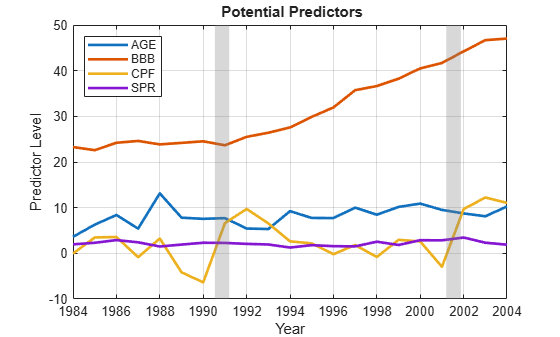
The potential predictors, measured for year t, are:
AGE Percentage of investment-grade bond issuers first rated 3 years ago. These relatively new issuers have a high empirical probability of default after capital from the initial issue is expended, which is typically after about 3 years.
BBB Percentage of investment-grade bond issuers with a Standard & Poor's credit rating of BBB, the lowest investment grade. This percentage represents another risk factor.
CPF One-year-ahead forecast of the change in corporate profits, adjusted for inflation. The forecast is a measure of overall economic health, included as an indicator of larger business cycles.
SPR Spread between corporate bond yields and those of comparable government bonds. The spread is another measure of the risk of current issues.
The response, measured for year t+1, is:
IGD Default rate on investment-grade corporate bonds
As described in [2] and [4], the predictors are proxies, constructed from other series. The modeling goal is to produce a dynamic forecasting model, with a one-year lead in the response (equivalently, a one-year lag in the predictors).
We first examine the data, converting the dates to a datetime vector so that the utility function recessionplot can overlay bands showing relevant dips in the business cycle:
% Convert dates to datetime vector:
dt = datetime(string(dates),'Format','yyyy');

% Plot potential predictors:
figure;
plot(dt,X0,'LineWidth',2)
recessionplot;
xlabel('Year')
ylabel('Predictor Level')
legend(predNames0,'Location','NW')
title('{\bf Potential Predictors}')
axis('tight')
grid('on')
% Plot response:
figure;
hold('on');
plot(dt,y0,'k','LineWidth',2);
plot(dt,y0-detrend(y0),'m--')
hold('off');
recessionplot;
xlabel('Year')
ylabel('Response Level')
legend(respName0,'Linear Trend','Location','NW')
title('{\bf Response}')
axis('tight');
grid('on');
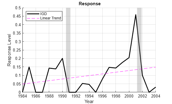
We see that BBB is on a slightly different scale than the other predictors, and trending over time. Since the response data is for year t + 1, the peak in default rates actually follows the recession in t = 2001.
Model Analysis
The predictor and response data can now be assembled into an MLR model, and the OLS estimate of can be found with the MATLAB backslash (\) operator:
% Add intercept to model:
X0I = [ones(T0,1),X0]; % Matrix
X0ITbl = [table(ones(T0,1),'VariableNames',{'Const'}),X0Tbl]; % Table

Estimate = X0I\y0
Estimate = 5×1

   -0.2274
    0.0168
    0.0043
   -0.0149
    0.0455
Alternatively, the model can be examined with LinearModel object functions, which provide diagnostic information and many convenient options for analysis. The function fitlm is used to estimate the model coefficients in from the data. It adds an intercept by default. Passing in the data in the form of a tabular array, with variable names, and the response values in the last column, returns a fitted model with standard diagnostic statistics:
M0 = fitlm(DataTable)
M0 =
Linear regression model:
    IGD ~ 1 + AGE + BBB + CPF + SPR

Estimated Coefficients:
                   Estimate        SE         tStat      pValue
                   _________    _________    _______    _________

    (Intercept)     -0.22741     0.098565    -2.3072     0.034747
    AGE             0.016781    0.0091845     1.8271     0.086402
    BBB            0.0042728    0.0026757     1.5969      0.12985
    CPF            -0.014888    0.0038077      -3.91    0.0012473
    SPR             0.045488     0.033996      1.338       0.1996


Number of observations: 21, Error degrees of freedom: 16
Root Mean Squared Error: 0.0763
R-squared: 0.621,  Adjusted R-Squared: 0.526
F-statistic vs. constant model: 6.56, p-value = 0.00253
There remain many questions to be asked about the reliability of this model. Are the predictors a good subset of all potential predictors of the response? Are the coefficient estimates accurate? Is the relationship between predictors and response, indeed, linear? Are model forecasts dependable? In short, is the model well-specified and does OLS do a good job fitting it to the data?
Another LinearModel object function, anova, returns additional fit statistics in the form of a tabular array, useful for comparing nested models in a more extended specification analysis:
ANOVATable = anova(M0)
ANOVATable=5×5 table
              SumSq      DF     MeanSq        F        pValue
             ________    __    _________    ______    _________

    AGE      0.019457     1     0.019457    3.3382     0.086402
    BBB      0.014863     1     0.014863      2.55      0.12985
    CPF      0.089108     1     0.089108    15.288    0.0012473
    SPR      0.010435     1     0.010435    1.7903       0.1996
    Error     0.09326    16    0.0058287
Summary
Model specification is one of the fundamental tasks of econometric analysis. The basic tool is regression, in the broadest sense of parameter estimation, used to evaluate a range of candidate models. Any form of regression, however, relies on certain assumptions, and certain techniques, which are almost never fully justified in practice. As a result, informative, reliable regression results are rarely obtained by a single application of standard procedures with default settings. They require, instead, a considered cycle of specification, analysis, and respecification, informed by practical experience, relevant theory, and an awareness of the many circumstances where poorly considered statistical evidence can confound sensible conclusions.
Exploratory data analysis is a key component of such analyses. The basis of empirical econometrics is that good models arise only through interaction with good data. If data are limited, as is often the case in econometrics, analysis must acknowledge the resulting ambiguities, and help to identify a range of alternative models to consider. There is no standard procedure for assembling the most reliable model. Good models emerge from the data, and are adaptable to new information.
Subsequent examples in this series consider linear regression models, built from a small set of potential predictors and calibrated to a rather small set of data. Still, the techniques, and the MATLAB toolbox functions considered, are representative of typical specification analyses. More importantly, the workflow, from initial data analysis, through tentative model building and refinement, and finally to testing in the practical arena of forecast performance, is also quite typical. As in most empirical endeavors, the process is the point.
References
[1] Cramér, H. Mathematical Methods of Statistics. Princeton, NJ: Princeton University Press, 1946.
[2] Helwege, J., and P. Kleiman. "Understanding Aggregate Default Rates of High Yield Bonds." Federal Reserve Bank of New York Current Issues in Economics and Finance. Vol. 2, No. 6, 1996, pp. 1–6.
[3] Kennedy, P. A Guide to Econometrics. 6th ed. New York: John Wiley & Sons, 2008.
[4] Loeffler, G., and P. N. Posch. Credit Risk Modeling Using Excel and VBA. West Sussex, England: Wiley Finance, 2007.
[5] Strang, G. Linear Algebra and Its Applications. 4th ed. Pacific Grove, CA: Brooks Cole, 2005.