Use the Fixed-Point Tool to Explore Numerical Behavior
This example shows how to use the Fixed-Point Tool to compare floating-point and fixed-point data types in your model. You can use the range collection functionality to explore and troubleshoot the numerical behavior of your model for different inputs.
Open the Fixed-Point Direct Form Filter Model
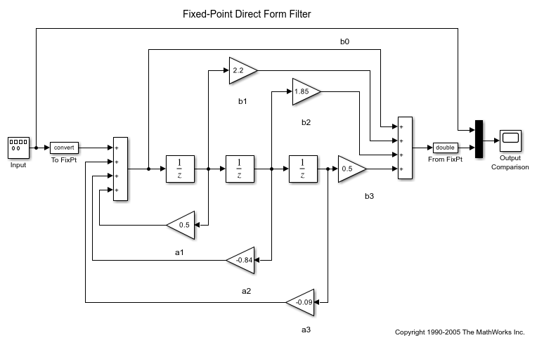
Open the fxpdemo_direct_form2 model. This tutorial uses a fixed-point direct form filter implemented using fundamental building blocks such as Gain, Delay, and Sum. The model contains a Signal Generator block that supplies a square wave input to the filter.
Set Up the Model
In this tutorial, you explore the behavior of the filter for a range of signal inputs.
To specify multiple simulation scenarios for range collection, define a Simulink.SimulationInput object in the base or model workspace. Define a
Simulink.SimulationInput object, simIn, that
specifies the amplitude of the square wave input for a range of
values.
simIn(1:6) = Simulink.SimulationInput('fxpdemo_direct_form2');

simIn(1) = simIn(1).setBlockParameter('fxpdemo_direct_form2/Input',...
    'Amplitude','0.001');
simIn(2) = simIn(2).setBlockParameter('fxpdemo_direct_form2/Input',...
    'Amplitude','0.01');
simIn(3) = simIn(3).setBlockParameter('fxpdemo_direct_form2/Input',...
    'Amplitude','0.1');
simIn(4) = simIn(4).setBlockParameter('fxpdemo_direct_form2/Input',...
    'Amplitude','1');
simIn(5) = simIn(5).setBlockParameter('fxpdemo_direct_form2/Input',...
    'Amplitude','10');
simIn(6) = simIn(6).setBlockParameter('fxpdemo_direct_form2/Input',...
    'Amplitude','100');
To specify signal tolerances, enable signal logging at the output of the Sum1 block.
Simulink.sdi.markSignalForStreaming('fxpdemo_direct_form2/Sum1',1,'on');
Open the Fixed-Point Tool and Collect Ranges
In the Apps tab of the
fxpdemo_direct_form2model, select Fixed-Point Tool.In the Fixed-Point Tool, click New > Range Collection.
Under System Under Design (SUD), select
fxpdemo_direct_form2.Under Range Collection Mode, select Simulation Ranges as the range collection method.
Under Simulation Inputs, select the
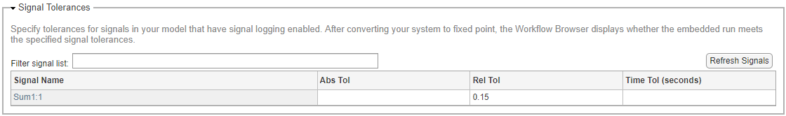
Simulink.SimulationInputobject,simIn, that you defined in the base workspace.To specify tolerances for the system, under Signal Tolerances, specify tolerances for any signal in the model with signal logging enabled.
Set the relative tolerance (Rel Tol) of the signal that you logged to 15%.
Under Collect Ranges, select
Double
                precision
.
When you collect ranges via simulation, the Fixed-Point Tool will override the data types in your model with doubles and simulate the model with instrumentation to collect minimum and maximum values for each object in your model. You can also choose to override data types with singles or scaled doubles, or use the current data type override set on the model.
Click the Collect Ranges button.
Simulink® simulates the
fxpdemo_direct_form2model six times, once for each amplitude of the input square wave specified in theSimulink.SimulationInputobject. The Fixed-Point Tool automatically enables fixed-point instrumentation and overrides the data types in your model with doubles to collect a floating-point baseline.You can view the ranges of each simulation individually by selecting the simulation scenario in the Workflow Browser.
Selecting the
BaselineRunnode in the Workflow Browser shows the merged ranges from the six simulation scenarios.
Click Settings, then select
Specified data types.Click Simulate with Embedded Types.
The Fixed-Point Tool simulates the model once for each simulation scenario, using the fixed-point data types specified in the model. Selecting the
EmbeddedRunnode in the Workflow Browser shows the merged results from the six simulation scenarios.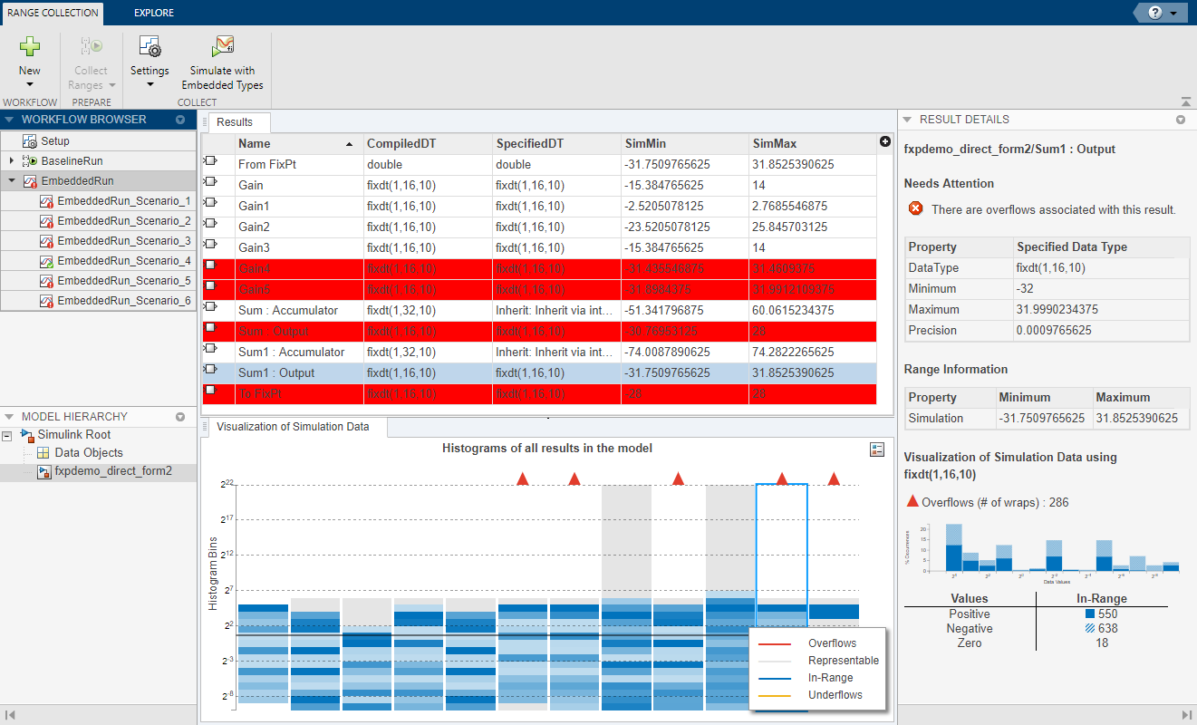
The Workflow Browser indicates that of the six simulation scenarios, only
EmbeddedRun_Scenario_4met the tolerances specified. Results with overflows are highlighted in red.
Explore Fixed-Point Behavior of the Model
Select the Explore tab of the Fixed-Point Tool to investigate further. Under Numerical Issues, select
Overflow, then click Execution Order.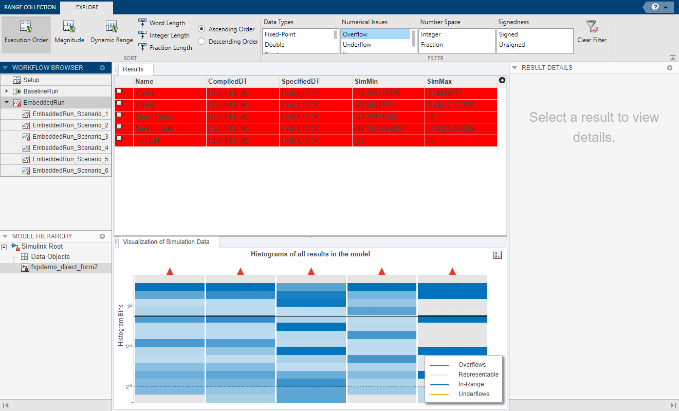
The Fixed-Point Tool displays only the
EmbeddedRunresults with overflows and sorts the list based on block execution order. In this example, the first overflow occurs in the Gain4 block.You can double-click any row in the Results spreadsheet to highlight the block in the model.
You can compare the fixed-point and floating-point behavior of the model for a specific simulation scenario using the Simulation Data Inspector. For example, the Fixed-Point Tool indicates that
EmbeddedRun_Scenario_3did not meet the specified tolerance. To compare this embedded run to the floating-point behavior for this simulation scenario, right-clickEmbeddedRun_Scenario_3and select Open Simulation Data Inspector to compare withBaselineRun_Scenario_3.
The Simulation Data Inspector plots the logged signal associated with the output of the
Sum1block forBaselineRun_Scenario_3andEmbeddedRun_Scenario_3, as well as their difference and the tolerance specified for this signal.
See Also
Propose Data Types for Merged Simulation Ranges | Control Views in the Fixed-Point Tool | Iterative Fixed-Point Conversion Using the Fixed-Point Tool