Use Frame-Based Data for Recursive Estimation in Simulink
This example shows how to use frame-based signals with the Recursive Least Squares Estimator block in Simulink®. Machine interfaces often provide sensor data in frames containing multiple samples, rather than in individual samples.
The recursive estimation blocks in the System Identification Toolbox™ accept these frames directly when you set Input Processing to Frame-based.
The blocks use the same estimation algorithms for sample-based and frame-based input processing. The estimation results are identical. There are some special considerations, however, for working with frame-based inputs in Simulink, and for visualizing the results.
This example is the frame-based version of the sample-based example in Estimate Parameters of System Using Simulink Recursive Estimator Block. The function reference for recursiveLS provides the equivalent sample-based command-line example.
System Description
The system has two parameters and is represented as:
 .
.
Here,
 and
and  are the real-time input and output data samples, respectively
 and
and  are the parameters
  .
. and
and  are the regressor samples. The regressor array
  is the row vector $${H_s} = \left[ {\matrix{ {u(t)} & {u(t - 1)} \cr } } \right]$.
Frame-Based Inputs
Data frames contain multiple data samples stacked in rows, with the last row containing the most recent data. For this example, each frame contains 10 samples. The observed inputs and outputs therefore arrive as ![$[u(1) ... u(10)]^T$](../../examples/ident/win64/UseFrameBasedDataWhenEstimatingRecursivelyInSimulinkRExample_eq09890455150590432786.png) and
and ![$[y(1) ... y(10)]^T$](../../examples/ident/win64/UseFrameBasedDataWhenEstimatingRecursivelyInSimulinkRExample_eq06779581039253211245.png) , where
, where  and
and  are the positions within the frame for a given time
  , and are equivalent to
  and
and  .
.
The regressor frame  also uses this stacking. The
  element in the upper right corner is the last sample from the previous input frame.
![$${H_f} = \left[ {\matrix{ {{u(1)}} & {{u(0)}} \cr {{u(2)}} & {{u(1)}} \cr \vdots & \vdots \cr {{u(10)}} & {{u(9)}} \cr } } \right]$$](../../examples/ident/win64/UseFrameBasedDataWhenEstimatingRecursivelyInSimulinkRExample_eq13013629441649193042.png)
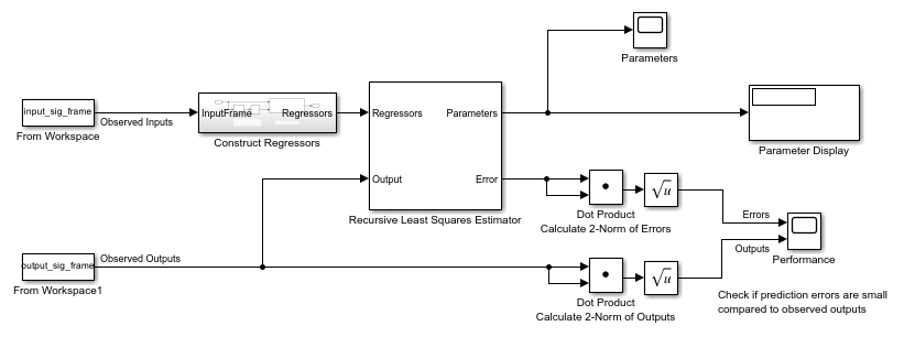
Open a preconfigured Simulink model based on the Recursive Least Squares Estimator block.
rlsfb = 'ex_RLS_Estimator_Block_fb';
open_system(rlsfb)
Observed Inputs and Outputs
Load the frame-based input and output signals into the workspace. Each signal consists of 30 frames, each frame containing ten individual time samples. In this implementation, the sample time is 1 second, and the frame time is 10 seconds.
load iddata3_frames input_sig_frame output_sig_frame
From Workspace blocks import signals that you loaded. In your application, this data may be arriving directly from your hardware.
Regressors
The model constructs the Regressors frame Hframe in the Construct Regressors subsystem, using input_sig_frame.
open_system([rlsfb '/Construct Regressors'])
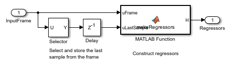
As Frame-Based Inputs described, the frame-based regressor signal consists of the all elements of the current frame of observed inputs, along with the last sample from the previous frame. The Selector block extracts the last sample from the observed inputs frame, and the Delay block stores this value for the next frame step.
Construct Regressors, a MATLAB Function block, constructs the signal Hframe. The first column of Hframe contains the current input frame. The second column contains the current frame, shifted by one position. The first element of the second column, representing the oldest sample, is from the previous observed inputs frame.
Recursive Least Squares Estimator Block
The block configuration includes frame-based input processing with a sample time of 10.
Error Visualization
The Error port provides the prediction errors in vector-valued frame ![$[e(1) ... e(10)]^T$](../../examples/ident/win64/UseFrameBasedDataWhenEstimatingRecursivelyInSimulinkRExample_eq08264190231711887556.png) , where
, where  is the position within the frame at a given time and is equivalent to
  . These prediction errors can be compared to observed outputs frame in multiple ways. This example compares the 2-norms of these vectors. An error vector with a small norm relative to the observed outputs norm suggests successful estimation. The scope displays a plot of the comparison.
Results
Run the simulation. The Parameters scope shows the progression of the  and
and  parameter estimates. The adjacent Parameter Display displays the current values of and . The scope Performance plots the 2-norms of the observed outputs and prediction error frames, as described in error as it compares with the original measurement signal as described in Error Visualization.
sim(rlsfb)
open_system([rlsfb '/Parameters'])
open_system([rlsfb '/Performance'])
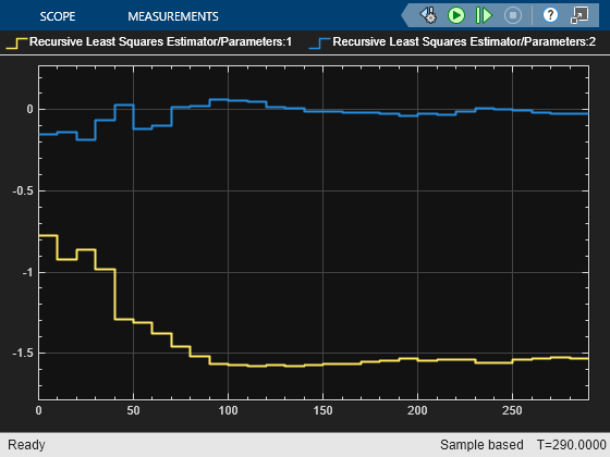
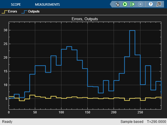
The Parameters plot shows that parameter estimates converge at approximately T = 150. The Performance plot shows that the prediction errors are small compared with the observed outputs. These results suggest a successful estimation. The final parameter estimates in the Parameter display are identical to those in the command-line and the sample-based Simulink examples linked at the beginning of this example.
See Also
Recursive Least Squares Estimator | Recursive Polynomial Model Estimator | recursiveLS