Build Map from 2-D Lidar Scans Using SLAM

This example uses:

This example shows you how to implement the simultaneous localization and mapping (SLAM) algorithm on a series of 2-D lidar scans using scan processing algorithms and pose graph optimization (PGO). The goal of this example is to estimate the trajectory of the robot and build a map of the environment.

The SLAM algorithm in this example incrementally processes the lidar scans and builds a pose graph to create the map of the environment. To overcome the drift accumulated in estimated robot trajectory, the example recognizes previously visited places through scan matching and utilizes the loop closure information to optimize poses and update the map of the environment. To optimize the pose graph, this example uses 2-D pose graph optimization from Navigation Toolbox™.

In this example, you learn how to:

Estimate robot trajectory from a series of scans using scan registration algorithms.
Optimize the drift in estimated robot trajectory by identifying previously visited places (loop closures).
Visualize the map of the environment using scans and their absolute poses.

Load Laser Scans

This example uses data collected in an indoor environment using a Jackal™ robot from Clearpath Robotics™. The robot is equipped with a SICK™ TiM-511 laser scanner with a maximum range of 10 meters. Load the offlineSlamData.mat file containing the laser scans into the workspace.

data = load('offlineSlamData.mat');
scans = data.scans;

Robot Trajectory Estimation

The example uses the matchScansGrid and matchScans functions to estimate the relative pose between successive scans. The matchScansGrid function provides the initial estimate for the relative pose, which is accurate up to the specified resolution. The matchScans function uses the estimate as an initial guess, and refines the relative pose for better estimation.

% Set maximum lidar range to be slightly smaller than maximum range of the
% scanner, as the laser readings are less accurate near maximum range
maxLidarRange = 8;
% Set the map resolution to 10 cells per meter, which gives a precision of
% 10cm
mapResolution = 10;
% Create a pose graph object and define information matrix
pGraph = poseGraph;
infoMat = [1 0 0 1 0 1];
% Loop over each scan and estimate relative pose
prevScan = scans{1};
for i = 2:numel(scans)
    currScan = scans{i};
    % Estimate relative pose between current scan and previous scan
    [relPose,stats] = matchScansGrid(currScan,prevScan, ...
        'MaxRange',maxLidarRange,'Resolution',mapResolution);
    % Refine the relative pose
    relPoseRefined = matchScans(currScan,prevScan,'initialPose',relPose);
    % Add relative pose to the pose graph object
    pGraph.addRelativePose(relPoseRefined,infoMat);
    ax = show(pGraph,'IDs','off');
    title(ax,'Estimated Robot Trajectory')
    drawnow
    prevScan = currScan;
end

Figure contains an axes object. The axes object with title Estimated Robot Trajectory contains 2 objects of type line.

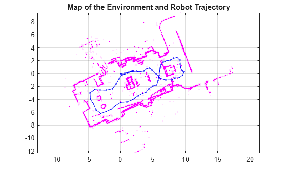
Notice that the estimated robot trajectory drifts over time. The drift can be due to any of the following reasons:

Noisy scans from the sensor without sufficient overlap
Absence of significant features
Inaccurate initial transformation, especially when rotation is significant

The drift in estimated trajectory results in an inaccurate map of the environment. Visualize the map and robot trajectory using the helperShow helper function, defined in the Supporting Functions section of this example.

hFigMap = figure;
axMap = axes('Parent',hFigMap);
helperShow(scans,pGraph,maxLidarRange,axMap);
title(axMap,'Map of the Environment and Robot Trajectory')

Figure contains an axes object. The axes object with title Map of the Environment and Robot Trajectory contains 72 objects of type line.

Drift Correction

Correct the drift in trajectory by accurately detecting the loops, which are places the robot has previously visited. Add the loop closure edges to the pose graph, which helps to correct the drift in trajectory during pose graph optimization.

Loop Closure Detection

Loop closure detection determines whether the robot has previously visited the current location. The search is performed by matching the current scan against the previous scans around the current robot location, within the radius specified by loopClosureSearchRadius. A scan is accepted as a match if the match score is greater than the specified loopClosureThreshold. Loop closures are detected using the helperDetectLoop helper function, which is attached to this example as a supporting file.

Adjust the loop closure parameters based on the quality of your results. You can increase the loopClosureThreshold value to reject false positives in loop closure detection, but the fuction might still return bad matches in environments with similar or repeated features. To address this, increase the loopClosureSearchRadius value to search a larger radius around the current pose estimate for loop closures, though this increases computation time.

loopClosureThreshold = 110;
loopClosureSearchRadius = 2;
[loopClosureEdgeIds,loopClosurePoses] = helperDetectLoop(scans,pGraph, ...
    loopClosureSearchRadius,loopClosureThreshold);

Trajectory Optimization

Add the detected loop closure edges to the pose graph to correct the drift in the estimated trajectory. Use the optimizePoseGraph (Navigation Toolbox) function to optimize the pose graph.

% Add loop closure edges to pose graph
if ~isempty(loopClosureEdgeIds)
    for k = 1:size(loopClosureEdgeIds,1)
        pGraph.addRelativePose(loopClosurePoses(k,:),infoMat, ...
            loopClosureEdgeIds(k,1),loopClosureEdgeIds(k,2));
    end
end
% Optimize pose graph
updatedPGraph = optimizePoseGraph(pGraph);

Visualization

Visualize the change in robot trajectory before and after pose graph optimization. The red lines represent loop closure edges.

hFigTraj = figure('Position',[0 0 900 450]);

% Visualize robot trajectory before optimization
axPGraph = subplot(1,2,1,'Parent',hFigTraj);
axPGraph.Position = [0.04 0.1 0.45 0.8];
show(pGraph,'IDs','off','Parent',axPGraph);
title(axPGraph,'Before PGO')

% Visualize robot trajectory after optimization
axUpdatedPGraph = subplot(1,2,2,'Parent',hFigTraj);
axUpdatedPGraph.Position = [0.54 0.1 0.45 0.8];
show(updatedPGraph,'IDs','off','Parent',axUpdatedPGraph);
title(axUpdatedPGraph,'After PGO')
axis([axPGraph axUpdatedPGraph],[-6 10 -7 3])
sgtitle('Robot Trajectory','FontWeight','bold')

Figure contains 2 axes objects and another object of type subplottext. Axes object 1 with title Before PGO contains 3 objects of type line. Axes object 2 with title After PGO contains 3 objects of type line.

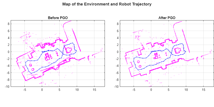
Visualize the map of the environment and robot trajectory before and after pose graph optimization.

hFigMapTraj = figure('Position',[0 0 900 450]);

% Visualize map and robot trajectory before optimization
axOldMap = subplot(1,2,1,'Parent',hFigMapTraj);
axOldMap.Position = [0.05 0.1 0.44 0.8];
helperShow(scans,pGraph,maxLidarRange,axOldMap)
title(axOldMap,'Before PGO')

% Visualize map and robot trajectory after optimization
axUpdatedMap = subplot(1,2,2,'Parent',hFigMapTraj);
axUpdatedMap.Position = [0.56 0.1 0.44 0.8];
helperShow(scans,updatedPGraph,maxLidarRange,axUpdatedMap)
title(axUpdatedMap,'After PGO')
axis([axOldMap axUpdatedMap],[-9 18 -10 9])
sgtitle('Map of the Environment and Robot Trajectory','FontWeight','bold')

Figure contains 2 axes objects and another object of type subplottext. Axes object 1 with title Before PGO contains 72 objects of type line. Axes object 2 with title After PGO contains 72 objects of type line.

Supporting Functions

The helperShow helper function visualizes the map of the environment and trajectory of the robot. The function transforms lidar scans using their corresponding poses to create a map of the environment.

function helperShow(scans,pGraph,maxRange,ax)
    hold(ax,'on')
    for i = 1:numel(scans)
        sc = transformScan(scans{i}.removeInvalidData('RangeLimits',[0.02 maxRange]), ...
            pGraph.nodes(i));
        scPoints = sc.Cartesian;
        plot(ax,scPoints(:,1),scPoints(:,2),'.','MarkerSize',3,'color','m')
    end
    nds = pGraph.nodes;
    plot(ax,nds(:,1),nds(:,2),'.-','MarkerSize',5,'color','b')
    hold(ax,'off')
    axis(ax,'equal')
    box(ax,'on')
    grid(ax,'on')
    xlabel('X')
    ylabel('Y')
end