Mixed-Signal Analyzer
Analyze circuit simulation data
Description
The Mixed-Signal Analyzer app enables you to visualize, analyze, and identify trends in mixed-signal simulation data. With the Cadence® Virtuoso ADE-MATLAB® Integration option you can import databases of circuit-level simulation results in MATLAB. To gain insights into the data, you can plot trends where you can vary different process parameters and see how the system behavior changes. You can compare the simulation results between different simulation runs and save and export your results.
Open the Mixed-Signal Analyzer App
MATLAB Toolstrip: In the Apps tab, under RF and Mixed-Signal, click the app icon.
MATLAB command prompt: Enter
mixedSignalAnalyzer.
Examples
Programmatic Use
More About
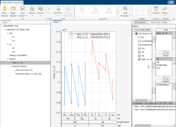
The Mixed-Signal Analyzer app reports the analysis results and metrics both as a plot and a metrics table in the Plot Options panel. If you select any data point in the figure, the corresponding data point in the metrics table is highlighted. Alternately, if you select any data point in the metrics table, the corresponding data point in the plot is highlighted.
You can select multiple data points and add legends to gain insight into their correlation. To select multiple data sets, hold the CTRL or the SHIFT button in your keyboard while selecting the data points.
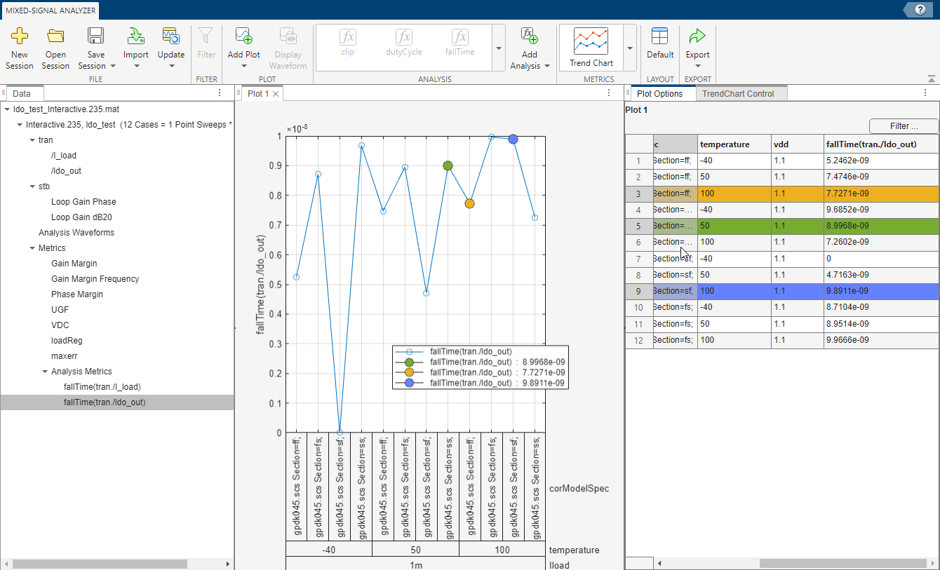
This allows you to easily map the data point in the figure to the data point in the metrics table for better insight about your design.