Accelerate Motion Planning with Deep-Learning-Based Sampler
The example shows how to use sampling-based planners such as RRT (rapidly-exploring random tree) and RRT* with Motion Planning Networks (MPNet), deep-learning-based sampler to find optimal paths efficiently.
The classical sampling-based planners such as RRT, RRT*, Bidirectional-RRT rely on generating samples from a uniform distribution over a specified state space. However, these planners typically restrict the actual robot path to a small portion of the state space. The uniform sampling causes the planner to explore many states which do not have an impact on the final path. This causes the planning process to become slow and inefficient, especially for state spaces with a large number of dimensions and environments that have narrow passages.
You can train a deep learning network to generate learned samples that can bias the path towards the optimal solution. Then, use the generated samples with the path planner to find the optimal paths in less computational time. The Train Deep Learning-Based Sampler for Motion Planning example shows how to train a MPNet to perform state space sampling.
Create Motion Planning Networks
Create a Motion Planning Networks object for SE(2) state space using mpnetSE2.
mpnet = mpnetSE2;
Load the trainedNetwork and the associated parameters from the .mat file, mazeMapTrainedMPNET.mat. The network is stored as a dlnetwork object with learned weights. The network was trained on various, randomly generated maze maps stored in MazeMapDataset.mat. The .mat file also contains optimal paths generated for random values of start and goal states in the training environments. The encodingSize is the size of the compressed representation of the maze map. The stateBounds specifies the bounds for the SE(2) state space.
load("mazeMapTrainedMPNET.mat","trainedNetwork","mazeParams","encodingSize","stateBounds")
Set the EncodingSize, Network, StateBounds properties of the mpnetSE2 object to the training environment values.
mpnet.EncodingSize = encodingSize;
mpnet.StateBounds = stateBounds;
mpnet.Network = trainedNetwork;
Create MPNet State Sampler
Create MPNet state sampler using state space and the MPNet object as inputs. Specify the limits for the maximum number of learned samples to 50.
stateSpace = stateSpaceSE2(stateBounds);
stateSamplerDL = stateSamplerMPNET(stateSpace,mpnet,MaxLearnedSamples=50,GoalThreshold=1);
Create Random Maze Map
Create a random maze map for testing the trained MPNet state sampler. picking a random start and goal from the map.
Click the Run button to generate a new map.
rng("default") %Set random seed
map = mapMaze(mazeParams{:});
figure
show(map)
![Figure contains an axes object. The axes object with title Binary Occupancy Grid, xlabel X [meters], ylabel Y [meters] contains an object of type image.](../../examples/deeplearning_shared/win64/AccelerateMotionPlanningWithDeepLearningBasedSamplerExample_03.png)
drawnow
Create state validator for the generated map. Set the validation distance to 0.1.
stateValidator = validatorOccupancyMap(stateSpace,Map=map);
stateValidator.ValidationDistance = 0.1;
Pick Random Start and Goal
Sample random start and goal from the map by specifying a minimum distance, minDistance between them. Choosing higher value of minDistance will make the motion planning more challenging as the start and goal points are far from each other and there can be more obstacles along the path. New start, goal pairs will be generated each time you click the Run button.
minDistance=
11; while true [start, goal] = sampleStartGoal(stateValidator); if distance(stateValidator.StateSpace, start,goal) >= minDistance break end end figure show(map); hold on plot(start(1),start(2),plannerLineSpec.start{:}) plot(goal(1),goal(2),plannerLineSpec.goal{:}) legend(Location="eastoutside")
![Figure contains an axes object. The axes object with title Binary Occupancy Grid, xlabel X [meters], ylabel Y [meters] contains 3 objects of type image, line. One or more of the lines displays its values using only markers These objects represent Start, Goal.](../../examples/deeplearning_shared/win64/AccelerateMotionPlanningWithDeepLearningBasedSamplerExample_04.png)
drawnow
Update Environment, StartState, and GoalState properties of the MPNet state sampler with the test map, start pose, and goal pose, respectively.
stateSamplerDL.Environment = map;
stateSamplerDL.StartState = start;
stateSamplerDL.GoalState = goal;
Plan RRT* Path
Run the following section or click PlanPath to generate the paths using uniform sampling and deep learning based sampling with MPNet.

Uniform Sampling
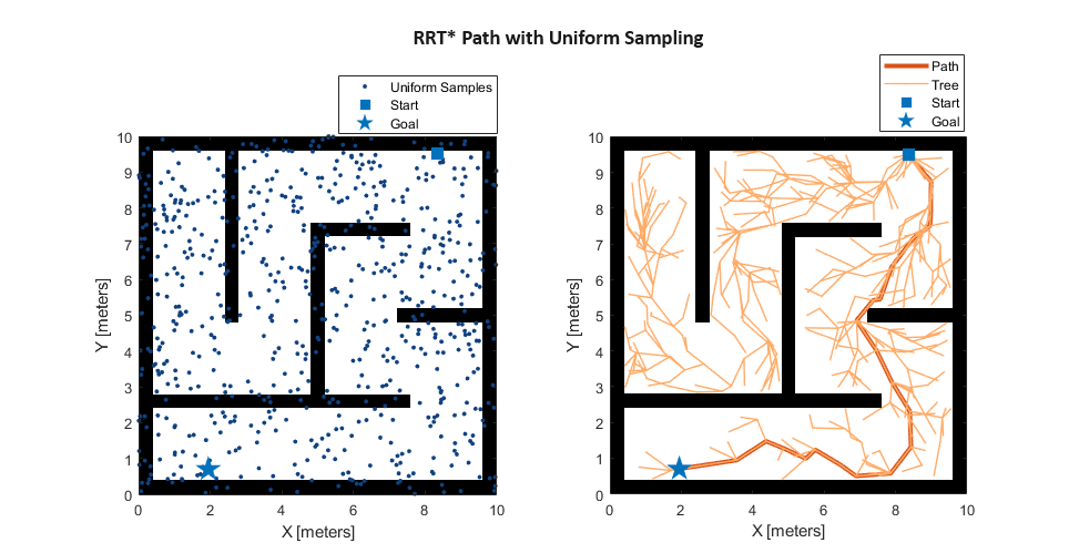
Plan a path with uniform state sampling. From the output, it is evident that the generated path is not smooth and the travel distance is not optimal due to the zigzag path. Also the RRT tree shows that many nodes are explored but are not used and they do not have any impact on the final path.
% Create RRT* planner with default uniform sampler
plannerUniformSampling = plannerRRTStar(stateSpace,stateValidator,MaxConnectionDistance=1,StateSampler=stateSamplerUniform(stateSpace));
[pathUniformSampling,solutionInfoUniformSampling] = plan(plannerUniformSampling,start,goal);

% Visualize results for uniform sampling
figure
show(map)
hold on;
plot(pathUniformSampling.States(:,1),pathUniformSampling.States(:,2),plannerLineSpec.path{:})
plot(solutionInfoUniformSampling.TreeData(:,1),solutionInfoUniformSampling.TreeData(:,2),plannerLineSpec.tree{:})
plot(start(1),start(2),plannerLineSpec.start{:});
plot(goal(1),goal(2),plannerLineSpec.goal{:});
legend(Location="northeastoutside")
title("Uniform sampling")
![Figure contains an axes object. The axes object with title Uniform sampling, xlabel X [meters], ylabel Y [meters] contains 5 objects of type image, line. One or more of the lines displays its values using only markers These objects represent Path, Tree, Start, Goal.](../../examples/deeplearning_shared/win64/AccelerateMotionPlanningWithDeepLearningBasedSamplerExample_05.png)
drawnow
MPNet Sampling
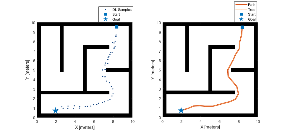
Plan a path with MPNet state sampling approach. From the output, it is evident that the generated path is smooth and the travel distance is much smaller than that of uniform sampling. Also the RRT tree shows that it sampler explores limited number of nodes that lie along a feasible optimal path between the start and goal points.
plannerDLSampling = plannerRRTStar(stateSpace,stateValidator,MaxConnectionDistance=1,StateSampler=stateSamplerDL);
[pathDLSampling,solutionInfoDLSampling] = plan(plannerDLSampling,start,goal);

% Visualize results with deep learning based sampling
figure
show(map);
hold on;
plot(pathDLSampling.States(:,1),pathDLSampling.States(:,2),plannerLineSpec.path{:})
plot(solutionInfoDLSampling.TreeData(:,1),solutionInfoDLSampling.TreeData(:,2),plannerLineSpec.tree{:})
plot(start(1),start(2),plannerLineSpec.start{:})
plot(goal(1),goal(2),plannerLineSpec.goal{:})
legend(Location="northeastoutside")
title("MPNet Sampling")
![Figure contains an axes object. The axes object with title MPNet Sampling, xlabel X [meters], ylabel Y [meters] contains 5 objects of type image, line. One or more of the lines displays its values using only markers These objects represent Path, Tree, Start, Goal.](../../examples/deeplearning_shared/win64/AccelerateMotionPlanningWithDeepLearningBasedSamplerExample_06.png)
drawnow
Performance Evaluation
Use plannerBenchmark to compare the performance of deep learning based sampling and uniform sampling using various evaluation metrics such as execution time, path length, smoothness. Choose the runCount to defines the number of runs to generate the metrics. Higher this value, the metrics are more accurate. There can be some scenarios where MPNet sampling perform worse than uniform sampling on some of these metrics, but the scenarios are less likley. In such cases, you can retrain the network to improve the accuracy.
% Number of runs to benchmark the planner runCount =30; % Create plannerBenchmark object pb = plannerBenchmark(stateValidator,start,goal); % Create function handles to create planners for uniform sampling and deep % learning-based sampling plannerUniformSamplingFcn = @(stateValidator)plannerRRTStar(stateValidator.StateSpace,stateValidator,MaxConnectionDistance=1); plannerMPNetSamplingFcn = @(stateValidator)plannerRRTStar(stateValidator.StateSpace,stateValidator,MaxConnectionDistance=1,StateSampler=stateSamplerDL); % Create plan function plnFcn = @(initOut,s,g)plan(initOut,s,g); % Added both planners to plannerBenchmark object addPlanner(pb,plnFcn,plannerUniformSamplingFcn,PlannerName="Uniform"); addPlanner(pb,plnFcn,plannerMPNetSamplingFcn,PlannerName="MPNet"); % Run planners for specified runCount runPlanner(pb,runCount)
Initializing Uniform ...
Done.
Planning a path from the start pose (0.51332 0.72885 -2.5854) to the goal pose (7.9835 9.4301 1.1543) using Uniform.
Executing run 1.
Executing run 2.
Executing run 3.
Executing run 4.
Executing run 5.
Executing run 6.
Executing run 7.
Executing run 8.
Executing run 9.
Executing run 10.
Executing run 11.
Executing run 12.
Executing run 13.
Executing run 14.
Executing run 15.
Executing run 16.
Executing run 17.
Executing run 18.
Executing run 19.
Executing run 20.
Executing run 21.
Executing run 22.
Executing run 23.
Executing run 24.
Executing run 25.
Executing run 26.
Executing run 27.
Executing run 28.
Executing run 29.
Executing run 30.
Initializing MPNet ...
Done.
Planning a path from the start pose (0.51332 0.72885 -2.5854) to the goal pose (7.9835 9.4301 1.1543) using MPNet.
Executing run 1.
Executing run 2.
Executing run 3.
Executing run 4.
Executing run 5.
Executing run 6.
Executing run 7.
Executing run 8.
Executing run 9.
Executing run 10.
Executing run 11.
Executing run 12.
Executing run 13.
Executing run 14.
Executing run 15.
Executing run 16.
Executing run 17.
Executing run 18.
Executing run 19.
Executing run 20.
Executing run 21.
Executing run 22.
Executing run 23.
Executing run 24.
Executing run 25.
Executing run 26.
Executing run 27.
Executing run 28.
Executing run 29.
Executing run 30.
Visualize Evaluation Metrics
Plot the metrics computed by plannerBenchmark. You can re-generate metrics for different maps, start and goal states.
The median executionTime for MPNet sampling is lower or similar to uniform sampling for most scenarios. However, MPNet sampling has less dispersion compared to uniform sampling. This makes the execution time more deterministic and suitable for real-time deployment.
figure
show(pb,"executionTime")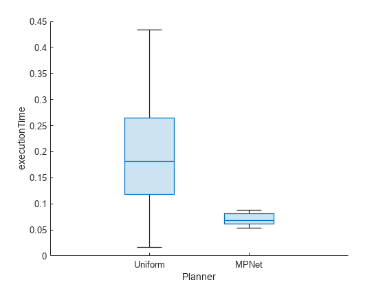
The pathLength is much smaller for MPNet sampling as compared to uniform sampling. Also, the dispersion is smaller which makes it more deterministic.
figure
show(pb,"pathLength")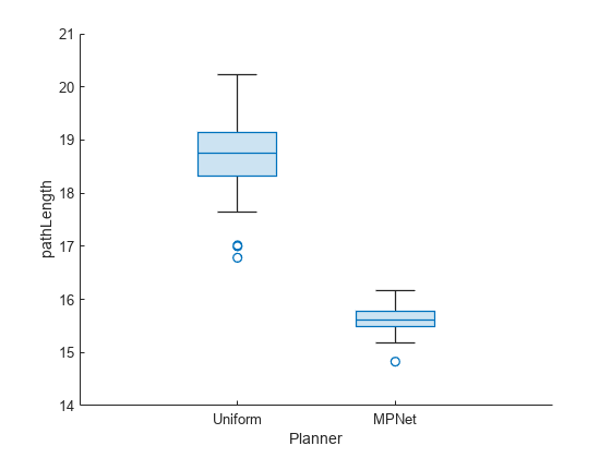
The smoothness is also much smaller for MPNet sampling when compared to uniform sampling. Also, the dispersion is smaller which makes it more deterministic.
figure
show(pb,"smoothness")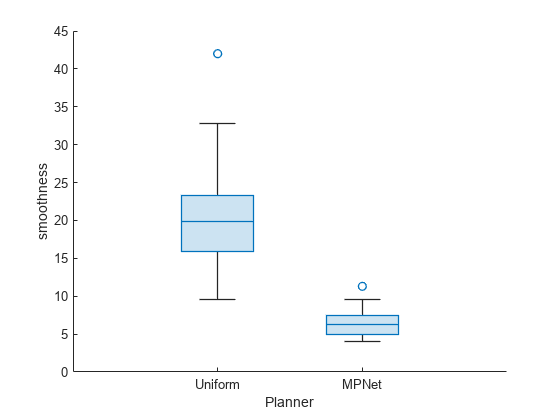
Plot the paths generated by the plannerBenchmark object for the specified runCount. We can observe that,
Uniform sampling gives paths that have high dispersion and are sub-optimal (they have higher path length and are less smooth).
MPNet sampling gives paths that have low dispersion and are near-optimal (they have smaller path length and are more smooth).
figure;
% Plot for planner output with uniform sampling
subplot(121)
show(map)
hold on
% Plot for planner output with MPNet sampling
subplot(122);
show(map)
hold on

for k =1:10
    runName = "Run" + num2str(k);

    % Planner output with uniform sampling
    subplot(121)
    pathStates = pb.PlannerOutput.Uniform.PlanOutput.(runName){1}.States;
    plot(pathStates(:,1),pathStates(:,2),DisplayName=runName)
    plot(start(1),start(2),plannerLineSpec.start{:})
    plot(goal(1),goal(2),plannerLineSpec.goal{:})
    title("Uniform sampling")

    % Planner output with MPNet sampling
    subplot(122)
    pathStates = pb.PlannerOutput.MPNet.PlanOutput.(runName){1}.States;
    plot(start(1),start(2),plannerLineSpec.start{:})
    plot(goal(1),goal(2),plannerLineSpec.goal{:})
    plot(pathStates(:,1),pathStates(:,2),DisplayName=runName)
    title("MPNet sampling")
end
![Figure contains 2 axes objects. Axes object 1 with title Uniform sampling, xlabel X [meters], ylabel Y [meters] contains 31 objects of type image, line. One or more of the lines displays its values using only markers These objects represent Run1, Start, Goal, Run2, Run3, Run4, Run5, Run6, Run7, Run8, Run9, Run10. Axes object 2 with title MPNet sampling, xlabel X [meters], ylabel Y [meters] contains 31 objects of type image, line. One or more of the lines displays its values using only markers These objects represent Start, Goal, Run1, Run2, Run3, Run4, Run5, Run6, Run7, Run8, Run9, Run10.](../../examples/deeplearning_shared/win64/AccelerateMotionPlanningWithDeepLearningBasedSamplerExample_10.png)
Conclusion
This example shows how to integrate the deep-learning-based sampler trained in the Train Deep Learning-Based Sampler for Motion Planning example with plannerRRTStar using a custom state sampler. It shows how the planned path and the RRT tree, improve with the learned sampling. It also shows the learned sampling gives statistically better performance for metrics such as execution time, path length and smoothness. We can use the deep-learning-based sampler approach for other sampling-based planners such as plannerRRT, plannerBiRRT, plannerPRM and we can also extend it for other applications such as manipulator path planning and UAV path planning.
See Also
mpnetSE2 | plannerRRTStar | stateSamplerMPNET | stateSamplerUniform
Topics
References
[1] Prokudin, Sergey, Christoph Lassner, and Javier Romero. “Efficient Learning on Point Clouds with Basis Point Sets.” In 2019 IEEE/CVF International Conference on Computer Vision Workshop (ICCVW), 3072–81. Seoul, Korea (South): IEEE, 2019. https://doi.org/10.1109/ICCVW.2019.00370.
[2] Qureshi, Ahmed Hussain, Yinglong Miao, Anthony Simeonov, and Michael C. Yip. “Motion Planning Networks: Bridging the Gap Between Learning-Based and Classical Motion Planners.” IEEE Transactions on Robotics 37, no. 1 (February 2021): 48–66. https://doi.org/10.1109/TRO.2020.3006716.
[3] Qureshi, Ahmed H., and Michael C. Yip. “Deeply Informed Neural Sampling for Robot Motion Planning.” In 2018 IEEE/RSJ International Conference on Intelligent Robots and Systems (IROS), 6582–88. Madrid: IEEE, 2018. https://doi.org/10.1109/IROS.2018.8593772.