mpnetSE2

Motion Planning Networks

Since R2023b

Description

The mpnetSE2 object stores Motion Planning Networks (MPNet) to use for state space sampling or motion planning. MPNet is a deep-learning-based approach that uses neural networks to perform informed sampling or motion planning. MPNet uses prior knowledge to find optimal states for motion planning. Using this object, you can:

• Load a pretrained MPNet, and use it for state space sampling or motion planning.

• Configure an untrained MPNet to train on a new data set. Then, use the trained MPNet for state space sampling or motion planning.

Use the predict function of the mpnetSE2 object to predict state samples between a start pose and goal pose in a known or unknown input environment. Use the loss function of the mpnetSE2 object to compute the losses while training the network.

Creation

Syntax

mpnet = mpnetSE2

mpnet = mpnetSE2(Name=Value)

Description

mpnet = mpnetSE2 returns an untrained MPNet to train and use for sampling the SE(2) state space or for motion planning. You can train this network on a data set by using the trainnet (Deep Learning Toolbox) function.

mpnet = mpnetSE2(Name=Value) specifies properties using one or more name-value arguments. You can specify the Network, StateBounds, LossWeights, and EncodingSize properties as name-value arguments.

Use the Network property to store a deep neural network that you can use to perform informed sampling or motion planning in an unknown or known environment.

• To perform state space sampling using a pretrained MPNet, use stateSamplerMPNET object.

• To perform motion planning using a pretrained MPNet, use plannerMPNET object and the associated plan function.

Note

To run this function, you will require the Deep Learning Toolbox™.

Properties

Network — Pretrained or untrained MPNet

dlnetwork object | LayerGraph object

Pretrained or untrained MPNet, specified as a dlnetwork (Deep Learning Toolbox) or layerGraph (Deep Learning Toolbox) object. By default, this property contains an untrained MPNet.

StateBounds — Limits of SE(2) state space variables

[-100 100; -100 100; -pi pi] (default) | 3-by-2 matrix of real values

Limits of SE(2) state space variables, specified as a 3-by-2 matrix of real values.

• The first row specifies the lower and upper bounds of the state variable x in meters.

• The second row specifies the lower and upper bounds of the state variable y in meters.

• The third row specifies the lower and upper bounds of the state variable θ in radians.

Data Types: double

LossWeights — Loss function weights

[1 1 1] (default) | three-element vector of real positive values

Loss function weights, specified as a three-element vector of real positive values for each state variable, x, y, and θ, of the SE(2) state space.

The training loss for MPNet is the weighted mean squared distance between the predicted states and the actual states. The loss function weights specify the weight value for each state space variable while computing the loss.

Data Types: single | double

EncodingSize — Size of encoded environment

[10 10] (default) | two-element vector of nonnegative integers | nonnegative scalar

Size of the encoded environment, specified as a two-element vector of nonnegative integers or a nonnegative scalar.

• If specified as a vector, the elements of the vector specify the size of the encoded environment in the x and y directions.

• If specified as a scalar, the object uses the specified value for both the x and y directions.

The encoded environment is a compact representation of the input maps. The function encodes the input maps using Basis Point Set (BPS) encoding approach presented in [1]. EncodingSize specifies the number of basis points to use for compact representation of input maps.

For example, if N_sv is the number of state variables defining the input state space and [E_x E_y] is the size of the encoded environment, then the size of the encoded environment and the number of inputs to the MPNet must satisfy this equation:

NumInputs = 2×(N_sv+1) + (Ex×Ey)

.

If you train the MPNet on only a single map environment, there is no need to encode the map. Because, encoding one environment will not affect network predictions. Hence, you can set the EncodingSize value to 0.

For correct results, the EncodingSize value must be set before training the network. You must not modify the EncodingSize value while configuring the mpnetSE2 object for inference.

Data Types: single | double

NumInputs — Number of inputs

108 (default) | positive integer

This property is read-only.

Number of inputs to the MPNet, stored as a positive integer. The default value is 108.

The number of inputs to the network is determined by the sum of the size of the encoded environment and the number of state space variables representing both the current state and the goal state. The current state and goal state are provided as inputs to the network in the form of x, y, cosθ, and sinθ. Therefore, the number of state space variables given as input to the network is 8. The default size of the encoded environment is 10-by-10. Hence, the default number of inputs to the network is (10×10)+8 = 108.

If the size of the encoded environment is specified as 0, the number of inputs to the network is 8.

Data Types: double

NumOutputs — Number of outputs

4 (default)

This property is read-only.

Number of outputs from the MPNet, stored as 4. The network outputs state space variables, x, y, cosθ, and sinθ, which represent the predicted next state.

Data Types: double

Object Functions

predict	Predict state samples using MPNet
loss	Compute loss between predicted states and actual states
copy	Create deep copy of mpnetSE2 object

Examples

Train MPNet on Single Map Environment

Train a Motion Planning Networks (MPNet), on a single map environment, for state space sampling. In the case of a single map environment, you use a fixed map for training and testing the network. Then, you can use the trained network to compute state samples between any start pose and goal pose on the map. First, you must configure an MPNet and train the network on a small data set. Use training loss to evaluate the network accuracy. If training the MPNet on a large training data set created using multiple map environments, you must also compute validation loss to fine-tune the network accuracy. For information on how to train the MPNet on multiple map environments for state space sampling, see Train Deep Learning-Based Sampler for Motion Planning.

Load and Inspect Training Data

Load the input map and the training data into the MATLAB® workspace.

data = load("singleTrainData.mat","trainData","map")

data = struct with fields:
    trainData: {100×1 cell}
          map: [1×1 binaryOccupancyMap]

map = data.map;

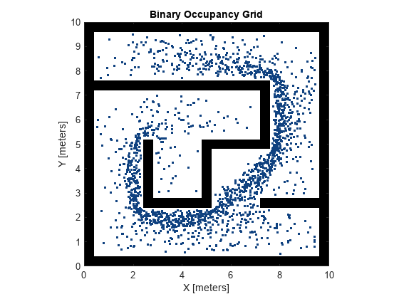
The training data consists of the optimal state samples computed for multiple, random values of start poses and goal poses on a maze map. Extract the training data from the data structure.

trainData = data.trainData;

Inspect the training data. The training data is a cell array of size 100-by-1 containing 100 state samples to use for training the network.

size(trainData)

ans = 1×2

   100     1

Read the state samples from the training data. Plot the input map and the training state samples.

figure
show(map)
hold on
for n = 1:100
    pathSample = trainData{n};
    plot(pathSample(:,1),pathSample(:,2),plannerLineSpec.state{:})
end
hold off

Create MPNet and Set Network Parameters

Create an untrained MPNet by using the mpnetSE2 object.

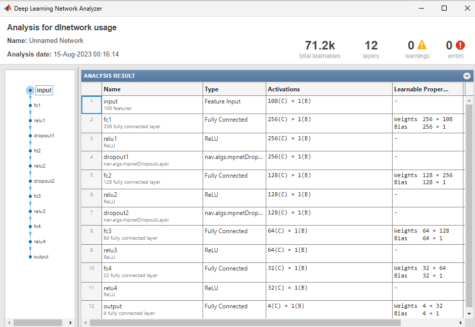
mpnet = mpnetSE2

mpnet = 
  mpnetSE2 with properties:

     StateBounds: [3×2 double]
     LossWeights: [1 1 1]
    EncodingSize: [10 10]
       NumInputs: 108
      NumOutputs: 4
         Network: [1×1 dlnetwork]

Visualize the network. To better understand the architecture of the network, inspect the layers in the network and number of inputs to each layer.

analyzeNetwork(mpnet.Network)

Set the StateBounds property of the mpnetSE2 object to the limits of the input map.

x = map.XWorldLimits;
y = map.YWorldLimits;
theta = [-pi pi];
stateBounds = [x; y; theta];
mpnet.StateBounds = stateBounds;

Set the EncodingSize property of the mpnetSE2 object to 0. This indicates that the function must not encode the input map to train the network. Setting the EncodingSize property to 0 changes the NumInputs property of the MPNet to 8.

mpnet.EncodingSize = 0

mpnet = 
  mpnetSE2 with properties:

     StateBounds: [3×2 double]
     LossWeights: [1 1 1]
    EncodingSize: [0 0]
       NumInputs: 8
      NumOutputs: 4
         Network: [1×1 dlnetwork]

Set the LossWeights property of the mpnetSE2 object to [10 10 0]. For higher weight values, the network takes more epochs for convergence. If the input is an SE(2) state space, the weight value for the state space variable $\theta$ is set to 0.

mpnet.LossWeights = [10 10 0];

Prepare Training Data

Prepare the training data by converting the samples in to a format required for training the MPNet. The mpnetPrepareData function rescales the values of the optimal path states to the range [0, 1] and stores them as a datastore object to use with the training function.

dsTrain = mpnetPrepareData(trainData,mpnet);

Train MPNet

Create a trainingOptions object for training the MPNet. These training options have been chosen experimentally. If you use a new data set for training, you must change your training options to achieve the desired training accuracy.

• Use the Adam optimizer.

• Set the size of training mini-batches to 20.

• Shuffle the training datastore at every epoch.

• Set the maximum number of epochs to 50.

options = trainingOptions("adam", ...
    MiniBatchSize=20, ...
    MaxEpochs=50, ...
    Shuffle="every-epoch", ...
    Plots="training-progress", ...   
    VerboseFrequency=500);

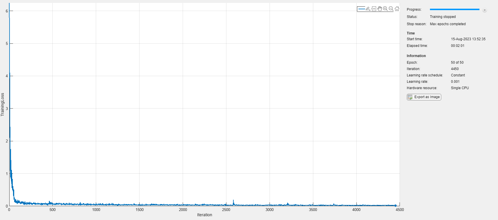
Train the MPNet by using the trainnet function. Specify the loss function and training options as inputs to the training function. For optimal results, the training loss must converge to zero.

[net,info] = trainnet(dsTrain,mpnet.Network,@mpnet.loss,options);

    Iteration    Epoch    TimeElapsed    LearnRate    TrainingLoss
    _________    _____    ___________    _________    ____________
            1        1       00:00:02        0.001          6.2466
          500        6       00:00:24        0.001        0.042451
         1000       12       00:00:38        0.001        0.073534
         1500       17       00:00:52        0.001        0.038856
         2000       23       00:01:04        0.001        0.041173
         2500       29       00:01:16        0.001        0.021427
         3000       34       00:01:28        0.001        0.044795
         3500       40       00:01:39        0.001        0.030961
         4000       45       00:01:50        0.001        0.028537
         4450       50       00:02:01        0.001        0.017648
Training stopped: Max epochs completed

Set the Network property of the mpnetSE2 object to the trained network.

mpnet.Network = net; 

Perform State Space Sampling Using Trained MPNet

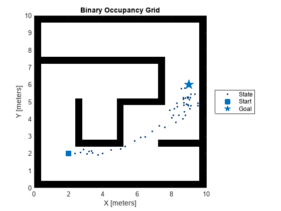
Specify a start pose and goal pose for which to compute state samples.

start= [2 2 0];
goal= [9 6 0];

Create a state space object for the specified state bounds.

stateSpace = stateSpaceSE2(stateBounds);

Configure the stateSamplerMPNet object to use the trained MPNet for state space sampling. Pass the map environment, start state, and goal state as inputs to the state sampler. Set the limits for maximum number of learned samples to consider to 50.

stateSamplerDL = stateSamplerMPNET(stateSpace,mpnet,Environment=map,StartState=start,GoalState=goal,MaxLearnedSamples=50);

Generate 50 state samples between the start and the goal poses.

samples = sample(stateSamplerDL,50);

Plot the generated state samples. Notice that the generated state samples are focused between the start and the goal states, and not scattered throughout the map environment. You can reduce the search time and find optimal paths quickly by using these state samples as seeds for motion planning.

figure
show(map)
hold on
plot(samples(:,1),samples(:,2),plannerLineSpec.state{:})
plot(start(1),start(2),plannerLineSpec.start{:})
plot(goal(1),goal(2),plannerLineSpec.goal{:})
legend(Location="eastoutside")

More Information

You can also save the trained MPNet to a .mat file for future use. Save the trained network, loss weights, and other network parameters to the .mat file. For information on how to use a pretrained network for state space sampling, see Predict State Samples Using MPNet Trained on Single Environment.

networkInput = mpnet.NumInputs;
networkOutput = mpnet.NumOutputs;
networkLossWeights = mpnet.LossWeights;
save("trainSingleMap.mat","net","map","networkInput","networkOutput","networkLossWeights");

Train MPNet on Custom Data for Motion Planning

This example shows how to train a MPNet on a custom dataset and then use the trained network for computing paths between two states in an unknown map environment.

Load and Visualize Training Data set

Load the data set from a .mat file. The data set contains 400,000 different paths for 200 maze map environments. The data set has been generated for a pre-defined parameters of mazeMap function. The first column of the data set contains the maps and the second column contains the optimal paths for randomly sampled start, goal states from the corresponding maps. The size of data set is 75MB.

% Download and extract the maze map dataset
if ~exist("mazeMapDataset.mat","file")
    datasetURL = "https://ssd.mathworks.com/supportfiles/nav/data/mazeMapDataset.zip";
    websave("mazeMapDataset.zip", datasetURL);
    unzip("mazeMapDataset.zip")
end

% Load the maze map dataset
load("mazeMapDataset.mat","dataset","stateSpace")
head(dataset)

             Map                  Path     
    ______________________    _____________

    1×1 binaryOccupancyMap    {14×3 single}
    1×1 binaryOccupancyMap    { 8×3 single}
    1×1 binaryOccupancyMap    {24×3 single}
    1×1 binaryOccupancyMap    {23×3 single}
    1×1 binaryOccupancyMap    {17×3 single}
    1×1 binaryOccupancyMap    {15×3 single}
    1×1 binaryOccupancyMap    { 7×3 single}
    1×1 binaryOccupancyMap    {10×3 single}

The data set was generated using the examplerHelperGenerateDataForMazeMaps helper function. The examplerHelperGenerateDataForMazeMaps helper function uses the mapMaze function to generate random maze maps of size 10-by-10 and resolution 2.5 m. The width and wall thickness of the maps was set to 5m and 1 m, respectively.

passageWidth = 5;
wallThickness = 1;
map = mapMaze(passageWidth,wallThickness,MapSize=[10 10],MapResolution=2.5)

Then, the start states and goal states are randomly generated for each map. The optimal path between the start and goal states are computed using plannerRRTStar path planner. The ContinueAfterGoalReached and MaxIterations parameters are set to true and 5000, respectively, to generate the optimal paths.

planner = plannerRRTStar(stateSpace,stateValidator); % Uses default uniform state sampling
planner.ContinueAfterGoalReached = true; % Optimize after goal is reached
planner.MaxIterations = 5000; % Maximum iterations to run the planner

Visualize a few random samples from the training data set. Each sample contains a map and the optimal path generated for a given start and goal state.

figure
for i=1:4
    subplot(2,2,i)
    ind = randi(height(dataset)); % Select a random sample
    map = dataset(ind,:).Map; % Get map from Map column of the table
    pathStates = dataset(ind,:).Path{1}; % Get path from Path column of the table
    start = pathStates(1,:);
    goal = pathStates(end,:);

    % Plot the data
    show(map);
    hold on
    plot(pathStates(:,1),pathStates(:,2),plannerLineSpec.path{:})
    plot(start(1),start(2),plannerLineSpec.start{:})
    plot(goal(1),goal(2),plannerLineSpec.goal{:})
end
legend(Location="bestoutside")

You can modify the helper function to generate new maps and train the MPNet from scratch. The dataset generation may take a few days depending upon CPU configuration and the number of maps you want to generate for training. To accelerate dataset generation, you can use Parallel Computing Toolbox™.

Create Motion Planning Networks

Create Motion Planning Networks (MPNet) object for SE(2) state space using mpnetSE2. The mpnetSE2 object loads a preconfigured MPNet that you can use for training. Alternatively, you can use the mpnetLayers function to create a MPNet with different number of inputs and hidden layers to train on the data set.

mpnet = mpnetSE2;

Set the StateBounds, LossWeights, and EncodingSize properties of the mpnetSE2 object. Set the StateBounds using the StateBounds property of the stateSpace object.

mpnet.StateBounds = stateSpace.StateBounds;

Specify the weights for each state space variables using the LossWeights property of the mpnetSE2 object. You must specify the weights for each state space variable $\mathit{x}$, $\mathit{y}$, and $\theta$ of SE(2) state space. For a SE(2) state space, we do not consider the robot kinematics such as the turning radius. Hence, you can assign zero weight value for the $\theta$ variable.

mpnet.LossWeights = [100 100 0];

Specify the value for EncodingSize property of the mpnetSE2 object as [9 9]. Before training the network, the mpnetSE2 object encodes the input map environments to a compact representation of size 9-by-9.

mpnet.EncodingSize = [9 9];

Prepare Data for Training

Split the dataset into train and test sets in the ratio 0.8:0.2. The training set is used to train the Network weights by minimizing the training loss, validation set is used to check the validation loss during the training.

split = 0.8;
trainData = dataset(1:split*end,:);
validationData = dataset(split*end+1:end,:);

Prepare the data for training by converting the raw data containing the maps and paths into a format required to train the MPNet.

dsTrain = mpnetPrepareData(trainData,mpnet);
dsValidation = mpnetPrepareData(validationData,mpnet);

Visualize prepared dataset. The first column of sample contains the encoded map data, encoded current state and goal states. The second column contains the encoded next state. The encoded state is computed as $[x,y,\cos (\theta ),\sin (\theta \left)\right]$ and normalized to the range of [0, 1].

preparedDataSample = read(dsValidation);
preparedDataSample(1,:)

ans=1×2 cell array
    {[0.2607 0.4112 0.6846 0.9647 0.9138 0.5757 0.4883 1.3733e-04 0.0549 0.1646 0 0.1646 0.1646 0.1646 0.1646 0.1646 0.0549 0.1646 0.8244 0.0870 0.9383 0.8244 0.8244 0.8244 0.8244 0.1646 0.1646 0.8244 0.0870 0.9020 0.0094 0.0870 0.0870 0.0870 3.9316e-16 0.1646 0.8244 0.0870 0.9020 0.0094 0.9020 0.9043 0.9383 0.1646 0.1646 0.8244 0.0870 0.9020 0.0094 0.9020 0.0870 0.8244 0.1646 0.1646 1 0.9043 0.9020 0.0094 0.9020 0.0870 0.8244 0.1646 0.1646 0.8313 0.0870 0.0870 0.0094 0.9020 0.0870 0.8244 0.1646 0.1646 0.9333 0.8244 0.8244 0.8244 0.9383 0.0870 0.8244 0.1646 0.0549 0.1646 0.1646 0.1646 0.1646 0.1646 2.6928e-16 0.1646 0.0549]}    {[0.2720 0.4130 0.6786 0.9670]}

Train Deep Learning Network

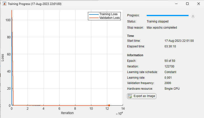
Use the trainnet function to train the MPNet. Training this network might take a long time depending on the hardware you use. Set the doTraining value to true to train the network.

doTraining = false;

Specify trainingOptions (Deep Learning Toolbox) for training the deep learning network:

• Set "adam" optimizer.

• Set the MiniBatchSize for training to 2048.

• Shuffle the dsTrain at every epoch.

• Set the MaxEpochs to 50.

• Set the ValidationData to dsValidation and ValidationFrequency to 2000.

You can consider the training to be successful once the training loss and validation loss converge close to zero.

if doTraining
    options = trainingOptions("adam",...
        MiniBatchSize=2048,...
        MaxEpochs=50,...
        Shuffle="every-epoch",...
        ValidationData=dsValidation,...
        ValidationFrequency=2000,...
        Plots="training-progress");

    % Train network
    [net,info] = trainnet(dsTrain,mpnet.Network,@mpnet.loss,options);

    % Update Network property of mpnet object with net
    mpnet.Network = net;
end

You can save the trained network and the details of input map environment to a .mat file and use it to perform motion planning. In the rest of example, you will use a pretrained MPNet to directly perform motion planning on an unknown map environment.

Load a .mat file containing the pretrained network. The network has been trained on various, randomly generated maze maps stored in the mazeMapDataset.mat file. The .mat file contains the trained network and details of the maze maps used for training the network.

if ~doTraining
    data = load("mazeMapTrainedMPNET.mat")
    mpnet.Network = data.trainedNetwork;
end

data = struct with fields:
      encodingSize: [9 9]
       lossWeights: [100 100 0]
        mazeParams: {[5]  [1]  'MapSize'  [10 10]  'MapResolution'  [2.5000]}
       stateBounds: [3×2 double]
    trainedNetwork: [1×1 dlnetwork]

Perform Motion Planning Using Trained MPNet

Create a random maze map for testing the trained MPNet for path panning. The grid size (MapSize×MapResolution) of the test map must be same the as that of the maps used for training the MPNet.

Click the Run button to generate a new map.

 
mazeParams = data.mazeParams;
map = mapMaze(mazeParams{:});
figure
show(map)

Create a state validator object.

stateValidator = validatorOccupancyMap(stateSpace,Map=map);
stateValidator.ValidationDistance = 0.1;

Create a MPNet path planner using the state validator and the MPNet object as inputs.

planner = plannerMPNET(stateValidator,mpnet);

Generate multiple random start and goal states by using the sampleStartGoal function.

[startStates,goalStates] = sampleStartGoal(stateValidator,500);

Compute distance between the generated start and goal states.

stateDistance=distance(stateSpace,startStates,goalStates);

Select two states that are farthest from each other as the start and goal for motion planning.

[dist,index] = max(stateDistance);
start = startStates(index,:);
goal = goalStates(index,:);

Plan path between the start and goal states using the trained MPNet.

[pathObj,solutionInfo] = plan(planner,start,goal)

pathObj = 
  navPath with properties:

      StateSpace: [1×1 stateSpaceSE2]
          States: [6×3 double]
       NumStates: 6
    MaxNumStates: Inf

solutionInfo = struct with fields:
        IsPathFound: 1
      LearnedStates: [32×3 double]
       BeaconStates: [2×3 double]
    ClassicalStates: [0×3 double]

Set the line and marker properties to display the start and goal states by using the plannerLineSpec.start and plannerLineSpec.goal functions, respectively.

sstate = plannerLineSpec.start(DisplayName="Start state",MarkerSize=6);
gstate = plannerLineSpec.goal(DisplayName="Goal state",MarkerSize=6);

Set the line properties to display the computed path by using the plannerLineSpec.path function.

ppath = plannerLineSpec.path(LineWidth=1,Marker="o",MarkerSize=8,MarkerFaceColor="white",DisplayName="Planned path");

Plot the planned path.

figure
show(map)
hold on
plot(pathObj.States(:,1),pathObj.States(:,2),ppath{:})
plot(start(1),start(2),sstate{:})
plot(goal(1),goal(2),gstate{:})
legend(Location="bestoutside")
hold off

Sample SE(2) State Space Using Pretrained MPNet

Load a data file containing a pretrained MPNet into the MATLAB workspace. The MPNet has been trained on randomly generated 2-D maze maps with widths and heights of 10 meters and a resolution of 2.5 cells per meter. The maze maps contain a passage width of 5 grid cells and wall thickness of 1 grid cell.

data = load("mazeMapTrainedMPNET.mat")

data = struct with fields:
      encodingSize: [9 9]
       lossWeights: [100 100 0]
        mazeParams: {[5]  [1]  'MapSize'  [10 10]  'MapResolution'  [2.5000]}
       stateBounds: [3x2 double]
    trainedNetwork: [1x1 dlnetwork]

Create a random maze map to use for motion planning. The grid size ($\mathrm{MapResolution}\times \mathrm{MapSize}$) must be the same as that of the maps used for training the MPNet.

rng(50,"twister")
map = mapMaze(5,1,MapSize=[20 20],MapResolution=1.25);

Specify the start pose and goal pose.

start = [2 8 0];
goal = [18 18 0];

Specify the state bounds, and create an SE(2) state space object.

x = map.XWorldLimits;
y =  map.YWorldLimits;
theta = [-pi pi];
stateBounds = [x; y; theta];
stateSpace = stateSpaceSE2(stateBounds);

Configure the mpnetSE2 object to use the pretrained MPNet for predicting state samples on a random map. Set the EncodingSize property values of the mpnetSE2 object to the values used for training the network.

mpnet = mpnetSE2(Network=data.trainedNetwork,StateBounds=stateBounds,EncodingSize=data.encodingSize);

Create an MPNet state sampler for computing the state samples. Specify the map environment and the start and goal poses as inputs to the state sampler.

mpnetSampler = stateSamplerMPNET(stateSpace,mpnet,Environment=map,StartState=start,GoalState=goal);

Generate 30 samples from the input state space for motion planning.

samples = sample(mpnetSampler,30);

Display the input map and plot the computed state samples.

figure
show(map)
hold on
plot(start(1),start(2),plannerLineSpec.start{:})
plot(goal(1),goal(2),plannerLineSpec.goal{:})
plot(samples(:,1),samples(:,2),plannerLineSpec.state{:})
legend(Location="bestoutside")
hold off

Plan Path Between Two States Using MPNet Path Planner

Load Pretrained MPNet

Load a data file containing a pretrained MPNet into the MATLAB® workspace. The MPNet has been trained on various 2-D maze maps with widths and heights of 10 meters and resolutions of 2.5 cells per meter. Each maze map contains a passage width of 5 grid cells and wall thickness of 1 grid cell.

data = load("mazeMapTrainedMPNET.mat")

data = struct with fields:
      encodingSize: [9 9]
       lossWeights: [100 100 0]
        mazeParams: {[5]  [1]  'MapSize'  [10 10]  'MapResolution'  [2.5000]}
       stateBounds: [3x2 double]
    trainedNetwork: [1x1 dlnetwork]

Set the seed value to generate repeatable results.

rng(10,"twister")

Create Maze Map for Motion Planning

Create a random maze map for motion planning. The grid size ($\mathrm{MapSize}\times \mathrm{MapResolution}$) must be same as that of the maps used for training the MPNet.

map = mapMaze(5,1,MapSize=[10 10],MapResolution=2.5);

Create State Validator

Create a state validator object to use for motion planning.

stateSpace = stateSpaceSE2(data.stateBounds);
stateValidator = validatorOccupancyMap(stateSpace,Map=map);
stateValidator.ValidationDistance = 0.1;

Select Start and Goal States

Generate multiple random start and goal states by using the sampleStartGoal function.

[startStates,goalStates] = sampleStartGoal(stateValidator,100);

Compute distance between the generated start and goal states.

stateDistance= distance(stateSpace,startStates,goalStates);

Select two states that are farthest from each other as the start and goal for motion planning.

[dist,index] = max(stateDistance);
start = startStates(index,:);
goal = goalStates(index,:);

Visualize the input map.

figure
show(map)
hold on
plot(start(1),start(2),plannerLineSpec.start{:})
plot(goal(1),goal(2),plannerLineSpec.goal{:})
legend(Location="bestoutside")
hold off

Compute Path Using MPNet Path Planner

Configure the mpnetSE2 object to use the pretrained MPNet for path planning. Set the EncodingSize property values of the mpnetSE2 object to that of the value used for training the network.

mpnet = mpnetSE2(Network=data.trainedNetwork,StateBounds=data.stateBounds,EncodingSize=data.encodingSize);

Create MPNet path planner using the state validator and the pretrained MPNet.

planner = plannerMPNET(stateValidator,mpnet);

Plan a path between the select start and goal states using the MPNet path planner.

[pathObj,solutionInfo] = plan(planner,start,goal);

Display Planned Path

Display the navPath object returned by the MPNet path planner. The number of states in the planned path and the associated state vectors are specified by the NumStates and States properties of the navPath object, respectively.

disp(pathObj)

  navPath with properties:

      StateSpace: [1x1 stateSpaceSE2]
          States: [5x3 double]
       NumStates: 5
    MaxNumStates: Inf

Set the line and marker properties to display the start and goal states by using the plannerLineSpec.start and plannerLineSpec.goal functions, respectively.

sstate = plannerLineSpec.start(DisplayName="Start state",MarkerSize=6);
gstate = plannerLineSpec.goal(DisplayName="Goal state",MarkerSize=6);

Set the line properties to display the computed path by using the plannerLineSpec.path function.

ppath = plannerLineSpec.path(LineWidth=1,Marker="o",MarkerSize=8,MarkerFaceColor="white",DisplayName="Planned path");

Plot the planned path.

figure
show(map)
hold on
plot(pathObj.States(:,1),pathObj.States(:,2),ppath{:})
plot(start(1),start(2),sstate{:})
plot(goal(1),goal(2),gstate{:})
legend(Location="bestoutside")
hold off

Display Additional Data

Display the solutionInfo structure returned by the MPNet path planner. This structure stores the learned states, classical states, and beacon states computed by the MPNet path planner. If any of these three types of states are not computed by the MPNet path planner, the corresponding field value is set to empty.

disp(solutionInfo)

        IsPathFound: 1
      LearnedStates: [50x3 double]
       BeaconStates: [2x3 double]
    ClassicalStates: [9x3 double]

Set the line and marker properties to display the learned states, classical states, and beacon states by using the plannerLineSpec.state.

lstate = plannerLineSpec.state(DisplayName="Learned states",MarkerSize=3);
cstate = plannerLineSpec.state(DisplayName="Classical states",MarkerSize=3,MarkerFaceColor="green",MarkerEdgeColor="green");
bstate = plannerLineSpec.state(MarkerEdgeColor="magenta",MarkerSize=7,DisplayName="Beacon states",Marker="^");

Plot the learned states, classical states, and beacon states along with the computed path. From the figure, you can infer that the neural path planning approach was unable to compute a collision-free path where beacon states are present. Hence, the MPNet path planner resorted to the classical RRT* path planning approach. The final states of the planned path constitutes states returned by neural path planning and classical path planning approaches.

figure
show(map)
hold on
plot(pathObj.States(:,1),pathObj.States(:,2),ppath{:})
plot(solutionInfo.LearnedStates(:,1),solutionInfo.LearnedStates(:,2),lstate{:})
plot(solutionInfo.ClassicalStates(:,1),solutionInfo.ClassicalStates(:,2),cstate{:})
plot(solutionInfo.BeaconStates(:,1),solutionInfo.BeaconStates(:,2),bstate{:})
plot(start(1),start(2),sstate{:})
plot(goal(1),goal(2),gstate{:})
legend(Location="bestoutside")
hold off

References

[1] Prokudin, Sergey, Christoph Lassner, and Javier Romero. “Efficient Learning on Point Clouds with Basis Point Sets.” In 2019 IEEE/CVF International Conference on Computer Vision Workshop (ICCVW), 3072–81. Seoul, Korea (South): IEEE, 2019. https://doi.org/10.1109/ICCVW.2019.00370.

[2] Qureshi, Ahmed Hussain, Yinglong Miao, Anthony Simeonov, and Michael C. Yip. “Motion Planning Networks: Bridging the Gap Between Learning-Based and Classical Motion Planners.” IEEE Transactions on Robotics 37, no. 1 (February 2021): 48–66. https://doi.org/10.1109/TRO.2020.3006716.

Extended Capabilities

C/C++ Code Generation

Generate C and C++ code using MATLAB® Coder™.

mpnetSE2 object properties must be compile-time constants.

Version History

Introduced in R2023b