Navigate Global Path Through Offroad Terrain Using Local Planner
This example shows how to use the model predictive path integral (MPPI) controller as a local planner that navigates planned network paths while conforming to the kinematic and geometric constraints of the haul truck. The example uses the road network path planner and road network derived from terrain data in the Create Route Planner for Offroad Navigation Using Digital Elevation Data example, and the terrain-aware global planner for entering and exiting that road network developed in the Create Onramp and Terrain-Aware Global Planners for Offroad Navigation example.
Load Terrain, Road Network, and Planner Parameter Data
Load the terrain data, road network paths, and planner parameters into the workspace.
addpath(genpath("Helpers"))
load("OpenPitMinePart1Data.mat","dem","pathList")              % Terrain and road network
load("OpenPitMinePart2Data.mat","originalReferencePath", ...   % Planned road network path
                                "smoothedReferencePath", ...   % Smoothed road network path
                                "fixedTerrainAwareParams", ... % Fixed terrain-aware parameters
                                "tuneableTerrainAwareParams")  % Tunable terrain-aware parameters
Use the exampleHelperDem2mapLayers helper function to convert the digital elevation data into a cost map.
[costMap,maxSlope] = exampleHelperDem2mapLayers(dem,tuneableTerrainAwareParams.MaxAngle,fixedTerrainAwareParams.Resolution);
obstacles = getLayer(costMap,"terrainObstacles");
Create MPPI Local Planner
While following the reference paths on the road network, the haul truck must be able to avoid collisions and stay as close to the reference paths as possible. To ensure this, you can use a model predictive path integral (MPPI) controller as a local planner. The controller samples local trajectories and computes from them an optimal trajectory using a cost function. The cost function attempts to follow the reference path while avoiding obstacles and enforcing smooth motions.
To create an MPPI controller, you must first define the parameters that describe the geometry and the kinematic constraints of the haul truck. The geometry parameters and kinematic constraints align with the two parameter categories used in the Create Onramp and Terrain-Aware Global Planners for Offroad Navigation example: those expected to stay constant during vehicle operation and those expected to change, respectively. Categorizing the parameters this way enables you to more easily incorporate your planning modules into a Simulink® model, as the separation aligns with how Simulink makes constant parameters accessible through block masks and accepts tunable parameters as Simulink bus signals.
Initialize the parameters for the local planner using the exampleHelperControllerParams example function. Note that you must keep the network planner parameters when setting the local planner parameters. For instance, you might choose the same minimum turning radius value for both planners, or opt for a larger radius in the network planner, to ensure that the local controller can follow the planned path more efficiently. This structured approach allows the MPPI controller to efficiently compute feasible and collision-free trajectories that the haul truck can follow in real-time, ensuring both obstacle avoidance and adherence to the reference paths.
[tunableControllerParams,fixedControllerParams] = exampleHelperControllerParams;
Initialize the vehicle dimensions using the defined parameters, and set up a collision checker with a specified inflation radius expanded from those dimensions.
vehDims = exampleHelperVehicleGeometry(fixedControllerParams.Length,fixedControllerParams.Width,"collisionChecker")vehDims =
vehicleDimensions with properties:
Length: 6.5000
Width: 5.7600
Height: 1.4000
Wheelbase: 6.5000
RearOverhang: 0
FrontOverhang: 0
WorldUnits: 'meters'
collisionChecker = inflationCollisionChecker(vehDims,3);
To ensure that the local planner can navigate the planned paths, inflate the road network by using the exampleHelperInflateRoadNetwork helper function.
exampleHelperInflateRoadNetwork(obstacles,pathList,collisionChecker.InflationRadius*1.5);
Create a local ego map that covers only the area accessible to the haul truck within one planning iteration of the local planner. This setup reduces the computational load required for the local planner to identify nearby obstacles, and minimizes the size of map signals for smoother integration into subsequent Simulink models.
maxDistance = tunableControllerParams.MaxVelocity(1)*tunableControllerParams.LookaheadTime;
localMap = occupancyMap(2*maxDistance,2*maxDistance,obstacles.Resolution);
localMap.GridOriginInLocal = -localMap.GridSize([2 1])/(2*localMap.Resolution);
Define the haul truck kinematics. Use a simple bicycle kinematics model to represent the haul truck. Configure the vehicle-specific parameters in the model.
vehicleObj = bicycleKinematics("VehicleInputs","VehicleSpeedHeadingRate");
vehicleObj.WheelBase = vehDims.Wheelbase;
maxForwardVel = tunableControllerParams.MaxVelocity(1);
maxReverseVel = -tunableControllerParams.MaxReverseVelocity;
vehicleObj.VehicleSpeedRange = [maxReverseVel maxForwardVel]; % [min, max velocity]
vehicleObj.MaxSteeringAngle = tunableControllerParams.MaxSteeringAngle;
Create the MPPI controller as an offroadControllerMPPI object using the smoothed network path and local ego map. This controller acts as the local planner. Now customize the controller parameters using the predefined properties.
mppi = offroadControllerMPPI(smoothedReferencePath,Map=localMap, VehicleModel=vehicleObj);
% Configure cost weight parameters
mppi.LookaheadTime = tunableControllerParams.LookaheadTime;
mppi.Parameter.ObstacleSafetyMargin = tunableControllerParams.ObstacleSafetyMargin; % In meters
mppi.Parameter.CostWeight.PathFollowing = tunableControllerParams.PathFollowingCost;
mppi.Parameter.CostWeight.PathAlignment = tunableControllerParams.PathAlignmentCost;
mppi.Parameter.CostWeight.ObstacleRepulsion = tunableControllerParams.ObstacleRepulsion;
mppi.Parameter.VehicleCollisionInformation = struct("Dimension", [vehDims.Length, vehDims.Width], "Shape", "Rectangle");
Simulate Haul Truck Following Reference Path
Simulate the haul truck driving along the reference path using the outputs from offroadControllerMPPI. The local planner generates optimal control commands [velocity angularVelocity] and the simulation integrates these commands to update the state of the haul truck. The control commands are evenly spaced in time with the interval set by the controller's SampleTime property.
Set Up Simulation Parameters
Initialize the parameters that you need for the simulation, such as the visualization interval and integration step size.
%% Follow path and visualize
curpose = mppi.ReferencePath(1,:);         % Current pose as first point in reference path
curvel = [0 0];                            % Current linear and angular velocity
simtime = 0;                               % Current simulation time starting at 0
tsReplan = 0.5;                            % Interval between re planning in seconds
tsIntegrator = 0.02;                       % Integration step size in seconds
tsVisualize = 0.1;                         % Visualization interval in seconds
itr = 0;                                   % Iteration counter
goalReached = false;                       % Flag for goal status
tVis = inf;                                % Time since last visualization
tPlan = inf;                               % Time since last planning
adjustedPath = 0;                          % Counter or flag for adjusted paths
Run Simulation
Set up the figures for the visualization. Convert obstacles to occupancyMap from binaryOccupancyMap because the offroadControllerMPPI runs faster with occupancyMap.
obstaclesMap = occupancyMap(obstacles.occupancyMatrix, obstacles.Resolution);
obstaclesMap.GridLocationInWorld = obstacles.GridLocationInWorld;
f = figure;
f.Visible = "on";
show(obstaclesMap);
hold on
exampleHelperPlotLines(mppi.ReferencePath,{"MarkerSize",10});
hControllerPath1_1 = quiver(nan,nan,nan,nan,.2,DisplayName="Current Path",LineWidth=3);

f = figure;
f.Visible = "on";
move(localMap,curpose(1:2),MoveType="Absolute");
syncWith(localMap,obstaclesMap);
h = show(localMap);
ax2 = h.Parent;
title("Simulation of Haul Truck Following Path")
hold on
Plot the original and smoothed reference paths.
exampleHelperPose2Quiver(originalReferencePath,{"AutoScale","off"});
exampleHelperPose2Quiver(mppi.ReferencePath,{"AutoScale","off"});
Initialize visualization for the offroadControllerMPPI path.
hRef = exampleHelperPlotLines(mppi.ReferencePath,{"MarkerSize",10});
hControllerPath1_2 = quiver(nan,nan,nan,nan,.2,DisplayName="Current Path");
[~,hVeh] = exampleHelperCreateVehicleGraphic(gca,"Start",collisionChecker);
hControllerPath2_2 = hgtransform;
arrayfun(@(x)set(x,"Parent",hControllerPath2_2),hVeh)
hRefCur = exampleHelperPlotLines(mppi.ReferencePath,".-");
To simulate and visualize the path-following behavior of a haul truck using the MPPI controller, follow these steps:
Update the local map and the state of the haul truck based on sensor inputs or global map information.
Periodically replan the path based on the current state of the haul truck, and visualize the updates.
Integrate the motion model of the haul truck over time to simulate movement.
End the simulation once the vehicle reaches the goal or meets a termination condition, such as encountering a local minima, that requires a new reference path.
% Simulate until haul truck is within 10 meters of the final goal position
while norm(curpose(1:2)-mppi.ReferencePath(end,1:2),2) > 10

    % Update visualization and local map if time since the last
    % visualization update exceeds the visualization interval
    if tVis >= tsVisualize
        move(localMap,curpose(1:2),MoveType="absolute",SyncWith=obstaclesMap);
        show(localMap,Parent=ax2,FastUpdate=1);
        hControllerPath2_2.Matrix(1:3,:) = [eul2rotm([0 0 curpose(3)],"XYZ") [curpose(1:2)';0]];
        drawnow limitrate;
        tVis = 0;
    end

    % Replan and update path of vehicle if time since last re-planning
    % exceeds re-planning time interval
    if tPlan >= tsReplan

        % Update local map
        move(localMap,curpose(1:2),MoveType="absolute",SyncWith=obstaclesMap);

        % Generate new velocity commands with MPPI controller
        [velcmds, curpath, info] = mppi(curpose, curvel);

        numCmds = size(velcmds,1);
        tstamps = (0:mppi.SampleTime: (numCmds-1)*mppi.SampleTime)';
        % End simulation if goal is reached
        if info.HasReachedGoal
            break
        end

        % Update MPPI path visualization with new state information
        set(hControllerPath1_1,XData=curpath(:,1), ...
                        YData=curpath(:,2), ...
                        UData=cos(curpath(:,3)), ...
                        VData=sin(curpath(:,3)))
        set(hControllerPath1_2,XData=curpath(:,1), ...
                        YData=curpath(:,2), ...
                        UData=cos(curpath(:,3)), ...
                        VData=sin(curpath(:,3)));
        set(hRefCur,XData=mppi.ReferencePath(:,1), ...
                    YData=mppi.ReferencePath(:,2))
        hControllerPath2_2.Matrix(1:3,:) = [eul2rotm([0 0 curpose(3)],"XYZ") [curpose(1:2)'; 0]];

        % Update simulation and visualization timestamps
        timestamps = tstamps + simtime;

        tVis = 0;
        tPlan = 0;
    end

    % Integrate the motion model
    simtime = simtime + tsIntegrator;
    tVis = tVis + tsIntegrator;
    tPlan = tPlan + tsIntegrator;

    % Compute the instantaneous velocity command to send to robot
    velcmd = velocityCommand(velcmds,timestamps,simtime);

    % Integrate the velocity command to find change in state
    statedot = derivative(vehicleObj, curpose, velcmd)';

    % Update current pose using the change in state
    curpose = curpose + statedot*tsIntegrator;

    % Update current velocity to the velocity command
    curvel = velcmd;
end
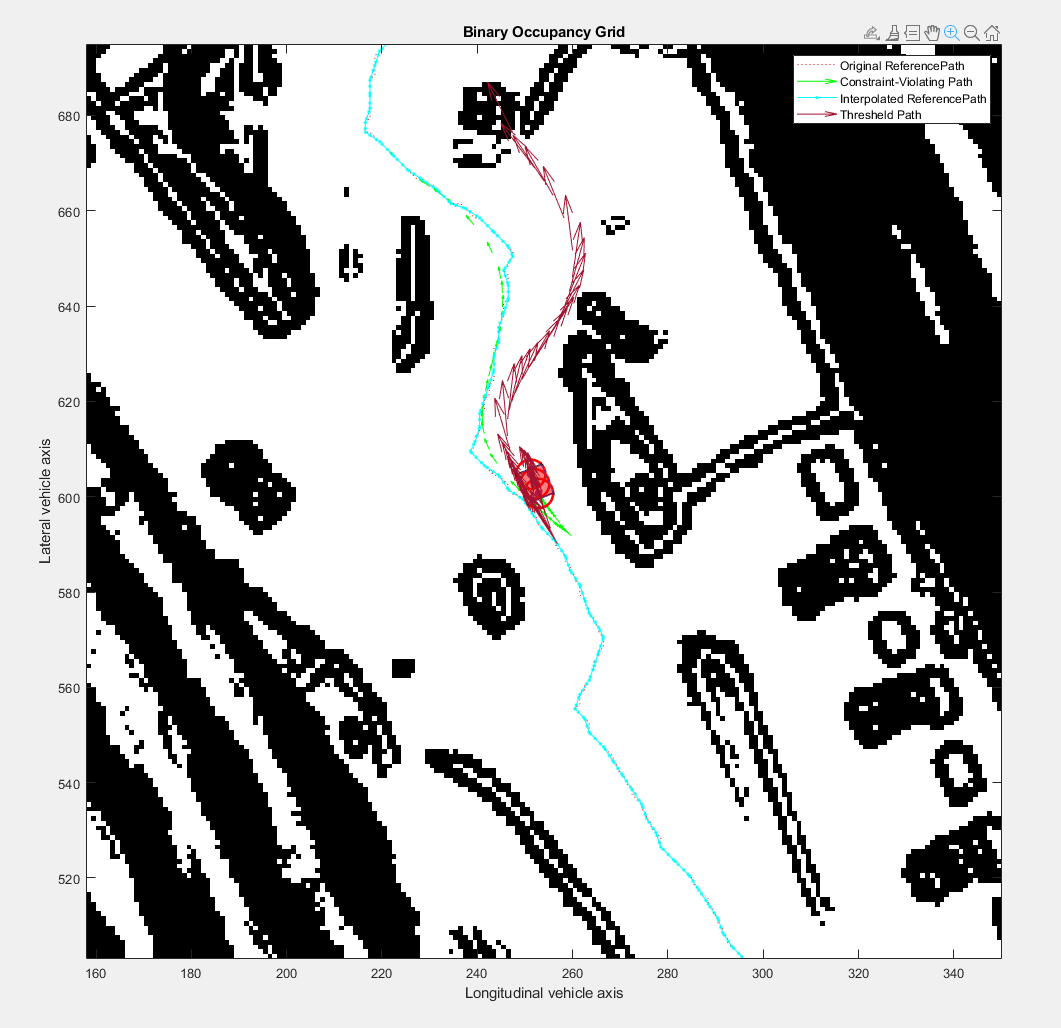
![Figure contains an axes object. The axes object with title Occupancy Grid, xlabel X [meters], ylabel Y [meters] contains 3 objects of type image, line, quiver. This object represents Current Path.](../../examples/offroad_autonomy/win64/NavigateGlobalPathThroughOffroadTerrainUsingLocalPlannerExample_02.png)
rmpath(genpath("Helpers"))Conclusion
This example showed how to use an MPPI-based local planner to guide a haul truck along a predefined off-road path while avoiding obstacles. The workflow covered configuring planner parameters, incorporating vehicle geometry and kinematic constraints, simulating the truck’s motion, and visualizing its trajectory.
Next, you can create a model predictive control (MPC) based controller to generate smoother control commands, as described in Create Path Following Model Predictive Controller example.
See Also
Topics
- Offroad Navigation for Autonomous Haul Trucks in Open Pit Mine
- Simulate Earth Moving with Autonomous Excavator in Construction Site