Parallel Language and Cluster Computing
Explain parfor errors with MATLAB Copilot
When the MATLAB® Code Analyzer app reports warnings or errors in a
parfor-loop, you can now use a MATLAB Copilot action to get a more detailed explanation of the issue. Copilot
explains the parfor requirement, guideline, or limitation
that the code violates, and it suggests changes to help resolve the error. To
use MATLAB Copilot, you must have a MATLAB Copilot license. For more information, see Resolve Issues in parfor-loops Using MATLAB Copilot.
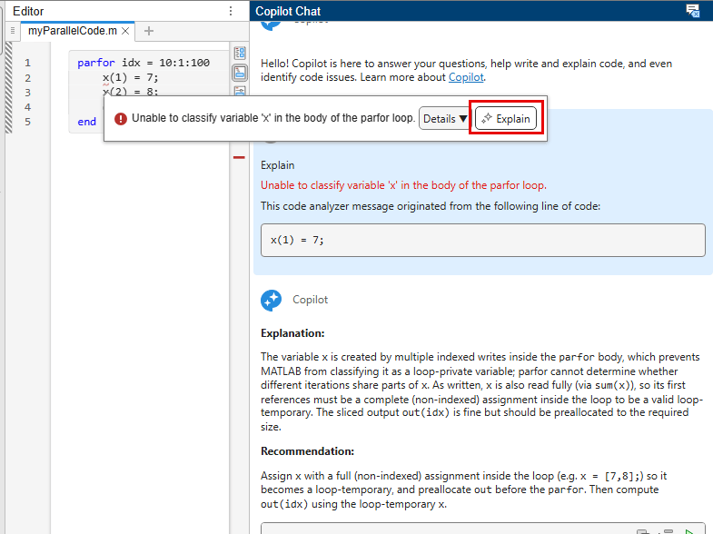
Explain parfor errors with MATLAB Copilot
Parallel Panel: Improved interface for managing your parallel computing environment
Use the Parallel panel to manage cluster profiles, discover clusters on your network or in the cloud, start and stop parallel pools, and select and monitor GPU devices. If the Parallel panel icon is not in the sidebar, click the Open more panels button . In the Open Panel dialog box that appears, select the Parallel panel.
For more information about using the panel to manage cluster profiles, see Discover Clusters and Use Cluster Profiles.
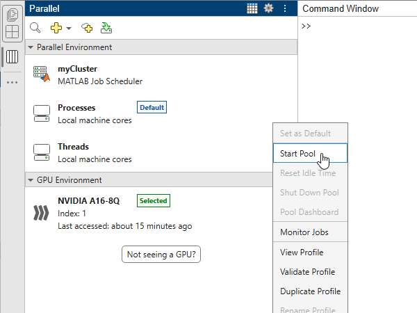
Parallel Panel: Improved interface for managing your parallel computing environment
Parallel Pools: Improved resilience to worker loss
Parallel pools can recover from worker loss without interrupting your computation. Parallel pool recovery is now supported on all cluster types. Previously, it was not supported on third-party scheduler clusters.
When you create an interactive or batch parallel pool, MATLAB starts the pool without Single Program Multiple Data (SPMD)
communication enabled, allowing the pool to recover from worker loss.
MATLAB enables SPMD communication automatically when required, such as
when you use spmd blocks or distributed arrays.
For more information, see How Parallel Pool Recovery Works.
Pool Dashboard: Select time range in Timeline
The Timeline graph of the Pool Dashboard now supports pan and zoom interactions that enable you to select regions of interest. When you zoom or pan to a time range in the Timeline graph, the Parallel Constructs, Summary, and Worker Summary tables display information about pool activity in the selected time range.
Run Signal Processing and Wavelet Functions on Thread Workers
Most Signal Processing Toolbox™ and Wavelet Toolbox™ functions now support thread-based environments. For full lists of supported functions, see Signal Processing Toolbox Functions with Thread Support (Signal Processing Toolbox) and Wavelet Toolbox Functions with Thread Support (Wavelet Toolbox).
For more information, see Run MATLAB Functions in Thread-Based Environment.
Improved memory usage for batch processing figures
When you create multiple figure windows using parallel workers, the figure windows now consume less memory than in previous releases. To further reduce memory usage, close any figures that you no longer need.
Distributed Arrays: Use functions with new and enhanced distributed array support
These functions have new and enhanced distributed array support:
conv2— You can now specify the input vectorsuandvas distributed arrays.
For more information, see Run MATLAB Functions with Distributed Arrays.
Tall Arrays: Use functions with new and enhanced tall array support
This function has enhanced tall array support:
unique— You can now use theTreatMissingAsDistinctname-value argument.
For more information, see Tall Arrays for Out-of-Memory Data.
MATLAB Job Scheduler: Control scripts accept double-dash option syntax
All MATLAB Job Scheduler control scripts now accept a double dash
(--) for command-line options, in addition to the
existing single dash (-) syntax.
Intel MPI Upgrade to Version "2021.17.0"
Parallel Computing Toolbox™ and MATLAB
Parallel Server™ now include an upgraded Intel® MPI Library, version "2021.17.0", for use on
Linux® for third-party schedulers.
To use Intel MPI, set the MPIImplementation additional
property for your third-party cluster profile or object to
"IntelMPI". To learn more about setting additional
properties, see Set Additional Properties (MATLAB Parallel Server).
Java Runtime no longer installed with MATLAB Parallel Server
MATLAB Parallel Server no longer includes Java® as part of its installation. Before R2026b, MATLAB Parallel Server installations on Windows® and Linux platforms included a Java Runtime Environment (JRE™).
MATLAB Job Scheduler Clusters
To start and run scheduler processes, MATLAB Job Scheduler requires a supported version of the JRE software. You can set MATLAB Job Scheduler to use your own JRE installation. Alternatively, you can allow MATLAB Job Scheduler to download and install a compatible OpenJDK® version by using the MATLAB Support for OpenJDK add-on. For more details, see Java Configuration for MATLAB Job Scheduler (MATLAB Parallel Server).
MATLAB Parallel Server Cluster Workers
MATLAB Parallel Server cluster workers no longer have access to JRE software. If you want cluster workers to run code that requires Java, you can configure your MATLAB Parallel Server installation to use any compatible JRE version installed on the cluster nodes. For details, see Configure MATLAB Parallel Server Workers to Use Java (MATLAB Parallel Server).
Admin Center: Simplified Tests for MATLAB Job Scheduler Cluster Connectivity
The Admin Center cluster connectivity tests for MATLAB Job Scheduler clusters are simplified. Admin Center now runs only Client to Nodes and Node to Nodes connectivity tests. Additionally, when you receive test failures, Admin Center now provides clear reasons for the failure and actionable next steps.
For example, these images show the connectivity tests in progress in each release.
| R2026a | R2026b |
|---|---|
|
|
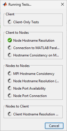
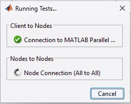
The Admin Center connectivity tests Client and Nodes to Client have been removed.
Functionality being removed or changed
parfor and mapreduce now throw
an error when automatic pool creation fails
Behavior change
If no parallel pool is open and automatic pool creation is enabled in your
parallel settings, then when automatic pool creation with the default
parallel environment fails, the parfor and mapreduce functions now throw
an error. You can use the error message to troubleshoot issues with pool
creation. In previous releases, the parfor and
mapreduce functions run in serial when automatic
pool creation fails.
In most cases, you do not need to make changes to your code if you
automatically start a parallel pool with the parfor or
mapreduce functions. However, if you do not want
parfor or mapreduce to throw
an error when MATLAB cannot automatically create a pool using the default parallel
environment, use one of these workarounds.
| Function | Example Code | Workaround |
|---|---|---|
parfor |
parfor(idx = 1:5) idx end |
try % Attempt to return current pool object or create a new pool object pool = gcp; catch Error warning("Failed to automatically create a parallel pool " + ... "with the default parallel environment. " + ... "Running serially on the client instead.") pool = gcp("nocreate"); % Otherwise create an empty pool object end parfor(idx = 1:5,pool) idx end |
mapreduce |
outds = mapreduce(ds,mapfun,reducefun); |
try % Attempt to return current pool object or create a new pool object pool = gcp; mr = mapreducer(pool); % Create ParallelMapReducer object catch Error warning("Failed to automatically create a parallel pool " + ... "with the default parallel environment. " + ... "Running serially on the client instead.") mr = mapreducer(0); % Otherwise, create a SerialMapReducer object end outds = mapreduce(ds,mapfun,reducefun,mr); |
Support for Windows Compute Cluster Server 2003, Windows HPC Server 2008, Windows HPC Server 2008 R2, Microsoft HPC Pack 2012, and Microsoft HPC Pack 2012 R2 has been removed
Errors
Support for these Microsoft® HPC schedulers has been removed:
Windows Compute Cluster Server 2003
Windows HPC Server 2008
Windows HPC Server 2008 R2
Microsoft HPC Pack 2012
Microsoft HPC Pack 2012 R2
If you use one of these schedulers, then to continue running MATLAB jobs on your cluster, update your HPC scheduler to Microsoft HPC Pack 2019.
For more information about configuring supported HPC Pack clusters to run MATLAB jobs, see Configure for Microsoft HPC Pack (MATLAB Parallel Server).
Additional configuration required for multi-release MATLAB Job Scheduler clusters
Behavior change
When you configure a MATLAB Job Scheduler cluster to run jobs with multiple MATLAB releases, supporting releases R2022b and earlier now requires additional configuration.
Before R2026b, you configure a MATLAB Job Scheduler cluster to support multiple MATLAB releases by using only the
MJS_ADDITIONAL_MATLABROOTS parameter. Starting in
R2026b, to support releases R2022b and earlier, you must also provide values
for these parameters in the mjs_def file on the head
node:
MJS_ADDITIONAL_SUPPORTED_RELEASES— Specify the supported older releases.MJS_LEGACY_JAVA— Specify a Java Runtime Environment (JRE) path for scheduler and worker processes. The JRE must be version 8 or 11.
For additional configuration steps, see Use Multiple MATLAB Parallel Server Releases in Cluster (MATLAB Parallel Server).
GPU Computing
Monitor GPU utilization, memory usage, and processes in real time
The GPU Monitor is an interactive tool for monitoring your GPU utilization, memory usage, and processes in real time. Monitor your GPU to verify that your code is running on the GPU and identify inefficiencies and bottlenecks in your GPU computing code.
With the GPU Monitor, you can:
Observe GPU utilization and memory usage during MATLAB computations. The monitor can plot these metrics for one GPU or for multiple GPUs simultaneously.
See which processes on your machine are using your GPUs.
Access GPU device information, including the state, capabilities, and driver version.
For information about how to interpret and respond to the metrics you see in the GPU Monitor, see Improve Performance Using GPU Monitor Metrics.
Pass GPU data to Python to improve performance of workflows that call Python from MATLAB
You can now use these functions to convert gpuArray data in
MATLAB to Python® GPU data types. These functions improve performance of GPU
workflows that call Python from MATLAB by removing the need to gather GPU data to host memory.
pycupyarray— converts an array in MATLAB to a CuPy array, if the CuPy module is installed in the Python environment.pydlpack— converts agpuArrayto a DLPack capsule.
You can also send GPU data from Python back to MATLAB by calling the gpuArray function on a CuPy
array or a DLPack capsule.
For more information about transferring GPU data between MATLAB and Python, see Pass GPU Data Between MATLAB and Python.
GPU Functionality in MATLAB: Use functions with new and enhanced gpuArray
support
These MATLAB and Parallel Computing Toolbox functions have new and enhanced gpuArray
support:
arrayfun— You can now use functions defined in a namespace witharrayfun. Using a namespace helps organize code and creates more robust names for the items contained inside it.norm— You can now calculate the generalized vector p-norm for0 < p < 1.parallel.gpu.RandStream.list— You can now specify an output argument to return a table of all available GPU generator algorithms. The table provides detailed information for each algorithm, including the generator name, multiple-stream support, and description.
For more information, see Run MATLAB Functions on a GPU. For a full list of MATLAB functions that accept GPU arrays, see Function List (GPU Arrays).
GPU Functionality in Signal Processing and Wireless Communications: Use
functions with new and enhanced gpuArray support
Signal Processing Toolbox
These Signal Processing Toolbox functions have new and enhanced gpuArray
support:
emd(Signal Processing Toolbox)vmd(Signal Processing Toolbox)chirp(Signal Processing Toolbox)tsa(Signal Processing Toolbox)tfridge(Signal Processing Toolbox) — Improved performance when extracting time-frequency ridges without a penalty for changing frequency.signalTimeFrequencyFeatureExtractor(Signal Processing Toolbox) — You can now use theemdandvmdtime-frequency analysis methods.
For a full list of Signal Processing Toolbox functions that accept GPU arrays, see Function List (GPU Arrays) (Signal Processing Toolbox).
Communications Toolbox
This Communications Toolbox™ function has new gpuArray support:
convenc(Communications Toolbox)
For a full list of Communications Toolbox functions that accept GPU arrays, see Function List (GPU Arrays) (Communications Toolbox).
DSP System Toolbox
These DSP System Toolbox™ System objects have new and enhanced gpuArray
support:
dsp.Channelizer(DSP System Toolbox)dsp.ChannelSynthesizer(DSP System Toolbox)dsp.FrequencyDomainFIRFilter(DSP System Toolbox)
For a full list of DSP System Toolbox functions that accept GPU arrays, see Function List (GPU Arrays) (DSP System Toolbox).
5G Toolbox
These 5G Toolbox™ functions have new gpuArray support:
nrTDLChannel(5G Toolbox)nrTimingEstimate(5G Toolbox)
For a full list of 5G Toolbox functions that accept GPU arrays, see Function List (GPU Arrays) (5G Toolbox).
GPU Functionality in Image Processing Toolbox: Use functions with new and enhanced gpuArray
support
These Image Processing Toolbox™ functions have new and enhanced gpuArray
support:
graythresh(Image Processing Toolbox)otsuthresh(Image Processing Toolbox)imerode(Image Processing Toolbox),imdilate(Image Processing Toolbox),imopen(Image Processing Toolbox),imclose(Image Processing Toolbox),imtophat(Image Processing Toolbox),imbothat(Image Processing Toolbox) — You can now use these functions to apply 3-D morphological operations using 3-D structuring elements.
For a full list of Image Processing Toolbox functions that accept GPU arrays, see Function List (GPU Arrays) (Image Processing Toolbox).
GPU Functionality in Deep Learning Toolbox: Speed up training using automatic mixed precision
This Deep Learning Toolbox™ function has enhanced GPU support:
trainnet(Deep Learning Toolbox) — You can now accelerate training and reduce memory usage on a GPU using automatic mixed precision. Set theTrainingPrecisionoption to"automatic-mixed"using thetrainingOptions(Deep Learning Toolbox) function to use half-precision floating-point arithmetic.
For a full list of Deep Learning Toolbox functions that accept GPU arrays, see Function List (GPU Arrays) (Deep Learning Toolbox).
GPU Functionality in Reinforcement Learning Toolbox: Set the UseGPUForLearning agent property to
calculate gradients using GPU
Agents in Reinforcement Learning Toolbox™ have this new property:
UseGPUForLearning— Set to"on"or"auto"to configure agents for GPU usage during training. This allows you to more easily configure the learnables, targets, and optimizers of an agent for GPU usage during training.
For more information, see Train Agents Using Parallel Computing and GPUs (Reinforcement Learning Toolbox).
Index into contiguous submatrices of sparse GPU arrays
You can now reference contiguous submatrices, that is, rectangular blocks of
adjacent elements of sparse gpuArray objects.
To access a submatrix of a sparse gpuArray, index into the
array using consecutive row and column indices. For example, access the central
3-by-3 submatrix of a 10-by-10 sparse gpuArray.
A = gpuArray.speye(10);
A(4:6,4:6)
  3×3 sparse gpuArray double matrix (3 nonzeros)

   (1,1)        1
   (2,2)        1
   (3,3)        1
For more information about indexing sparse GPU arrays, see Work with Sparse Arrays on a GPU.
GPU Workflow Example: Accelerate seismic migration using CUDA code
This new example shows how to accelerate your code by implementing long-running parts in CUDA® code and using advanced CUDA features, including cooperative groups:
Matrix-Matrix Multiplication: Improved performance on Blackwell GPUs
Matrix-matrix multiplication of gpuArray data shows
improved performance on Linux with NVIDIA® Blackwell architecture GPUs (compute capability 10.0 to 12.0). For
example, multiplying two 8192-by-8192 matrices on a Blackwell GPU is about 10.3x
faster than in R2026a.
function t = timeMatrixMultiply

% Reset GPU and set random number generator.
reset(gpuDevice);
gpurng("default");

% Create random matrices on GPU.
n = 8192;
A = rand(n,"gpuArray");
B = rand(n,"gpuArray");

% Time matrix multiplication.
t = gputimeit(@() A*B)
end
The approximate execution times are:
R2026a: 0.71 s
R2026b: 0.069 s
The code was timed on a Linux, Debian® 13.5, AMD® EPYC 9115 16-core processor @ 2.6 GHz test system with 64 GB of
memory and an NVIDIA RTX Pro 6000 GPU by calling the
timeMatrixMultiply function.
The performance improvement you observe will depend on your GPU hardware.
Sparse arrays: Improved performance when creating sparse GPU arrays
Creating a sparse gpuArray by calling the sparse function on a dense
gpuArray shows improved performance. For example,
calling sparse on a 10000-by-10000 dense
gpuArray is about 12x faster than in the previous
release.
function t = timeSparseGpuArray

% Reset GPU and set random number generator.
reset(gpuDevice);
gpurng("default")

% Create dense gpuArray.
sz = 10000;
dense = rand(sz,sz,"gpuArray");

% Time creating sparse gpuArray.
f = @() sparse(dense);
t = gputimeit(f)
end
The approximate execution times are:
R2026a: 0.349 s
R2026b: 0.029 s
The code was timed on a Windows 11, AMD EPYC 7262 8-core processor @ 3.2 GHz test system with 64 GB of
memory and an NVIDIA RTX A5000 GPU by calling the timeSparseGpuArray
function.
The performance improvement you observe will depend on your GPU hardware.
GPU computing in MATLAB upgraded to CUDA 13.1
GPU computing in MATLAB now uses CUDA 13.1. You can use new CUDA features when you write custom CUDA code for running in MATLAB via
mexcuda and parallel.gpu.CUDAKernel.
Maxwell, Pascal, and Volta architecture (compute capability 5.0 to 7.0) GPUs are no longer supported. For more information, see Support for Maxwell, Pascal, and Volta architecture GPUs is removed.
The supported version of the CUDA toolkit is now version 13.1. For more information, see Change to supported CUDA Toolkit.
Functionality being removed or changed
Support for Maxwell, Pascal, and Volta architecture GPUs is removed
Errors
Starting in R2026b, Maxwell, Pascal, and Volta architecture (compute capability 5.0 to 7.0) GPUs are no longer supported. The supported range of compute capabilities is 7.5 to 12.x.
For more information, see GPU Computing Requirements.
Change to supported CUDA Toolkit
Errors
CUDA Toolkit version 12.8 is no longer supported.
Recompile any MEX functions and PTX code that were compiled using the
mexcudafunction in previous versions of MATLAB.If you previously installed the CUDA Toolkit, install CUDA Toolkit version 13.1 instead.
For more information, see Install CUDA Toolkit (Optional).
Change to parallel.gpu.RandStream.list
Behavior change
Calling parallel.gpu.RandStream.list without an output argument now
displays a table of all available GPU generator algorithms, with more
detailed information about each algorithm: its name, whether it has
multiple-stream support, and a description. In previous releases,
parallel.gpu.RandStream.list displayed only the
available generator algorithms and their descriptions.
Change to supported PTX files for CUDA kernels
Errors
Creating a CUDAKernel object using the parallel.gpu.CUDAKernel
function from a PTX file compiled using PTX ISA version 3.0 or earlier is no
longer supported.
Recompile your PTX files using the mexcuda function.
mexcuda -ptx myCUFile.cu
Parallel Language and Cluster Computing
Parallel Computing Onramp: Free, self-paced, interactive course
Parallel Computing Onramp is a free, self-paced, interactive course that helps you get started with accelerating your MATLAB code using parallel computing.
Parallel Computing Onramp features hands-on exercises using MATLAB in your web browser. The course teaches you to:
Create and modify parallel pools.
Convert
forloops intoparforloops.Explore variable classification in
parforloops.Explore how parallel overhead impacts execution time.
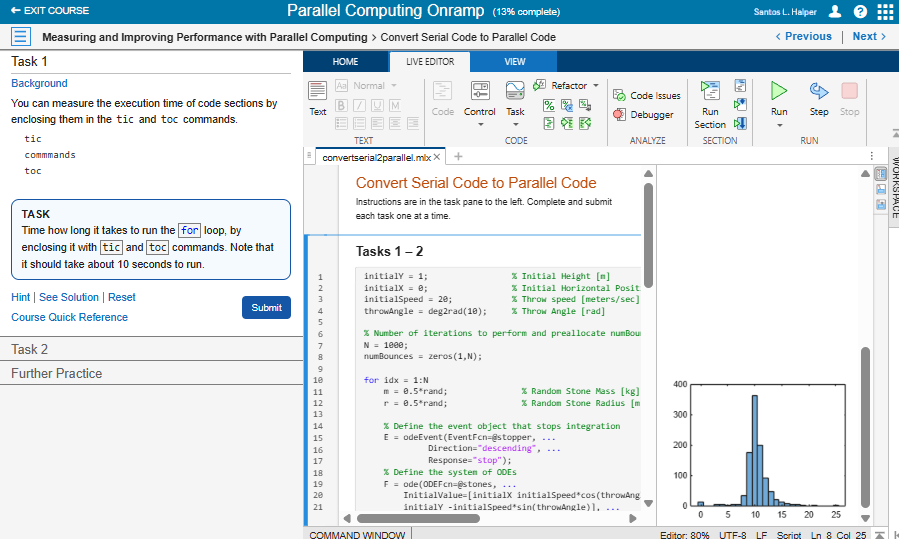
Parallel Computing Onramp: Free, self-paced, interactive course
parfor-Loops: Use consecutive decreasing integers as
loop index variables
You can now use consecutive decreasing integers as loop index variables in a
parfor-loop. Using such
variables allows you to simplify code that requires reverse iteration.
For example, this parfor-loop uses reverse iteration to
square values of n between 10 and 1. The loop index variable
n has a step value of
-1.
parfor n = 10:-1:1
  out(n) = n^2;
end
parfor-loop iterations
in a nondeterministic order.Thread-Based Parallel Pool: Monitor pool activity with Pool Dashboard
Use the Pool Dashboard to collect and visualize monitoring data for thread-based parallel pools. For more information, see Pool Dashboard.
You can also use a command line interface to collect pool activity monitoring
data on thread-based interactive parallel pools. For details, see parallel.pool.ActivityMonitor.
Thread-Based Environment: Use new functionality on thread workers
These MATLAB functions and objects now have thread-based support.
For more information, see Run MATLAB Functions in Thread-Based Environment.
Pool Dashboard: Run code directly in Pool Dashboard
Run and monitor MATLAB code directly from the Pool Dashboard using the Enter code to run and monitor box. For an example that shows how to use the Enter code to run and monitor box, see Investigate parfor -Loop with Pool Dashboard.
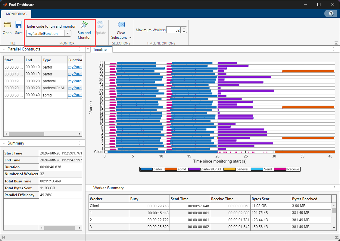
Pool Dashboard: Run code directly in Pool Dashboard
Local Parallel Pools: Support for more than 64 workers on Windows 11
You can now create local parallel pools with more than 64 workers on
Windows 11 machines that have more than 64 cores. The default number of
workers for local parallel pools you create with the Threads
and Processes profiles on a multicore Windows 11 machine is now equal to the number of physical cores. In previous
releases, MATLAB creates local pools with only 64 workers even on machines with
more cores.
Cluster Profile Manager: View additional NumWorkers
property information for local profiles
The Cluster Profile Manager now displays how MATLAB determines the default value of the
NumWorkers property of the Processes
and Threads profiles, unless you have modified this property.
This insight helps you understand the default maximum number of workers
available for a local parallel pool, especially on CPUs that have both
performance and efficiency cores.
The Cluster Profile Manager now also shows the number of physical cores
MATLAB detects on your computer, as well as the number of performance
cores, if any. To view this information, point to the information button
 next to the
 NumWorkers property
value.
For more information about how MATLAB sets the default number of workers for local parallel environments, see Determine Default Pool Size for Local Parallel Environments.
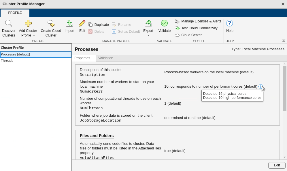
Cluster Profile Manager: View additional NumWorkers property information for local profiles
Cluster Validation: Validate cluster object
You can now validate parallel.Cluster objects using
the validate object function. You can specify which validation
stages to run, set the number of workers to use, and write the validation
results to a file.
Cluster Profiles: Delete profiles programmatically
Use the parallel.deleteProfile function to delete cluster profiles
programmatically.
Parallel Workflows: New Examples and Topics
Use these new examples to learn about parallel computing:
Optimize Parallel Pools for Multithreaded Computations — This example shows how to tune the number of threads per worker to improve the computational performance of your parallel pool.
Control and Repeat Random Numbers in Parallel Jobs — This example shows how to control random number generation for independent jobs and tasks.
Monitor During Parallel Optimizations with
parfor— This example shows how to useparforto run multiple optimization problems in parallel, while monitoring solver progress on the client.Monitor During Parallel Optimizations with
parfeval— This example shows how to perform multiple optimizations in parallel withparfevaland monitor the progress on the client.Monitor and Stop Optimization Running On Worker — This example shows how to run an optimization on a parallel worker and stop it early from the client without losing intermediate results.
Communicate Between Workers in SPMD Computations — This example shows how to exchange data between workers during
spmdcomputations using thespmdSendandspmdReceivefunctions.Fit Distributed Logistic Regression Using
drange— This example shows how to use distributed arrays andfor-drange-loops to implement logistic regression on large data.Compute Parallel Prefix Scans with SPMD Computations — This example shows how to implement a reusable, scalable, SPMD based prefix scan using a parallel workers.
Use these new topics to learn about parallel computing:
Determine Default Pool Size for Local Parallel Environments — Learn how MATLAB automatically sets the default number of workers for local parallel environments.
Resolve Error: Client Lost Connection to Worker — Troubleshoot lost connection to worker errors when running code on parallel pools.
Cloud Center: Streamlined user interface for creating and using MATLAB Parallel Server clusters
MATLAB Parallel Server on Cloud Center has a new user interface and underlying infrastructure. The operating system is updated to Ubuntu® 24.04, providing improved performance, security, and user experience.
The configuration settings for the cloud machine configuration in Cloud Center are adapted from the MATLAB Parallel Server on Amazon Web Services reference architecture available on GitHub®.
Cloud Clusters: Promote and demote parallel jobs
MATLAB Parallel Server on AWS: Customize and deploy your own Amazon Machine Image
You can now customize and build your own Linux Amazon® Machine Image (AMI) for running MATLAB Parallel Server on AWS®, using the same scripts that form the basis of the build process for MathWorks prebuilt images. A HashiCorp® Packer® template generates the machine image.
To build your own machine image using MathWorks scripts, see the build scripts and instructions on GitHub for customizing and deploying your own AMI.
Cluster Administration: Simplify MATLAB Job Scheduler cluster connectivity using SOCKS5 Proxy
You can now use a SOCKS5 proxy server to streamline connectivity between
MATLAB clients and MATLAB Job Scheduler clusters. The new
parallelserverproxy tool forwards all Parallel Computing Toolbox network traffic through a single endpoint. This capability reduces
the need for multiple open ports and simplifies firewall and network
configurations, especially for clients outside the cluster’s virtual network or
in cloud and hybrid environments. The parallelserverproxy
also authenticates clients using mutual TLS and encrypts communication between
the MATLAB clients and cluster.
For more information, see Configure SOCKS5 Proxy for MATLAB Job Scheduler (MATLAB Parallel Server).
Support for MPICH: Use MPICH version 4.2.3
Parallel Computing Toolbox and MATLAB Parallel Server now come with MPICH version 4.2.3 for use on Linux and Mac operating systems.
Cluster Administration: New and updated troubleshooting topics
Use these new and updated topics to resolve issues with MATLAB Job Scheduler and MATLAB Parallel Server in third-party scheduler clusters.
Resolve Communication Issues in MATLAB Job Scheduler Cluster (MATLAB Parallel Server) — Troubleshoot common issues related to hostname resolution and connectivity within your MATLAB Job Scheduler cluster.
Resolve Memory Errors on Linux Clusters (MATLAB Parallel Server) — Troubleshoot out of memory errors caused by system limits on Linux operating systems.
Resolve Scaling Issues in the Cloud (MATLAB Parallel Server) - Troubleshoot MATLAB Parallel Server scaling issues in the cloud.
Tall Arrays: Improved performance when joining tables
The join and
innerjoin functions show
improved performance when the first input is a tall table. The second input
argument can be an in-memory table or the result of a reduction operation on a
tall table. For details, see the tall array performance improvements described
in the MATLAB release notes.
Distributed Arrays: Use functions with new and enhanced distributed array support
These functions have new distributed array support:
These functions have enhanced distributed array support:
isbetween— You can now use theDataVariablesandOutputFormatname-value arguments and specify distributed tables and timetables as input arguments.ichol— You can now specify nonsymmetric and non-hermitian matrices as input.movmad,movmax,movmean,movmedian,movmin,movprod,movstd,movsum, andmovvar— You can now use these functions with distributed tables and timetables.
For more information, see Run MATLAB Functions with Distributed Arrays.
Functionality being removed or changed
addAttachedFiles now updates already attached
files
Behavior change
The addAttachedFiles function
now updates files that are already attached to the parallel pool. In
previous releases, the addAttachedFiles function did
not update already attached files.
GPU Computing
Support for Blackwell GPU Architectures: Update to NVIDIA CUDA 12.8
Parallel Computing Toolbox now uses CUDA version 12.8, which supports NVIDIA GPUs with compute capability up to 12.x, including Blackwell architecture GPUs. For more information, see GPU Computing Requirements.
CUDA Toolkit version 12.2 is no longer supported. Recompile any MEX
functions and PTX code that were compiled using the mexcuda function in
previous versions of MATLAB. For more information, see Change
to supported CUDA Toolkit.
GPU Functionality in MATLAB: Use functions with new and enhanced gpuArray
support
These MATLAB functions have new gpuArray support:
fminsearch— This function now accepts GPU arrays but does not run on a GPU.strings— This function now accepts GPU arrays but does not run on a GPU.
These MATLAB functions have enhanced gpuArray
support:
besseli— You can now specify negative equation orders.expm— You can now use this function with diagonal sparsegpuArrayobjects.issorted— You can now determine if the elements of the first column of agpuArraymatrix are sorted in ascending order by using the'rows'option. If a column contains repeated elements, then theissortedfunction uses the ordering of the elements in the next column to the right to determine the sorting order.kron— You can now use this function with sparsegpuArrayobjects.ldivide— You can now divide sparsegpuArrayobjects by a scalar.max,min— You can now return the maximum or minimum value of a sparsegpuArrayobject by using the"all"option.plus,+— You can now append agpuArrayobject to a string without first callinggatheron thegpuArrayobject.
For more information, see Run MATLAB Functions on a GPU. For a full list of MATLAB functions that accept GPU arrays, see Function List (GPU Arrays).
GPU Functionality in Statistics and Machine Learning Toolbox: Use functions with new and enhanced gpuArray
support
These Statistics and Machine Learning Toolbox™ functions have new and enhanced gpuArray
support:
cvpartition(Statistics and Machine Learning Toolbox) — You can now partition data for cross-validation. The object functionsrepartition(Statistics and Machine Learning Toolbox),summary(Statistics and Machine Learning Toolbox),test(Statistics and Machine Learning Toolbox), andtraining(Statistics and Machine Learning Toolbox) accept the resultingcvpartitionobject and can also execute on a GPU.fitrgp(Statistics and Machine Learning Toolbox) — You can now fit a Gaussian process regression (GPR) model. Most object functions of the modelsRegressionGP(Statistics and Machine Learning Toolbox),CompactRegressionGP(Statistics and Machine Learning Toolbox), andRegressionPartitionedGP(Statistics and Machine Learning Toolbox) now support GPU array input arguments. The functions that do not arelime(Statistics and Machine Learning Toolbox) andshapley(Statistics and Machine Learning Toolbox).fitdist(Statistics and Machine Learning Toolbox),mle(Statistics and Machine Learning Toolbox) — You can now fit Rician distributions to data and estimate the maximum likelihood of Rician distributions.fitcecoc(Statistics and Machine Learning Toolbox) — You can now specify kernel learners when you create aCompactClassificationECOC(Statistics and Machine Learning Toolbox) orClassificationPartitionedKernelECOC(Statistics and Machine Learning Toolbox) model object usingfitcecoc.ncx2cdf(Statistics and Machine Learning Toolbox),ncx2pdf(Statistics and Machine Learning Toolbox),ncx2inv(Statistics and Machine Learning Toolbox),ncx2stat(Statistics and Machine Learning Toolbox)shapley(Statistics and Machine Learning Toolbox),fit(Statistics and Machine Learning Toolbox) — Theshapley(Statistics and Machine Learning Toolbox) andfit(Statistics and Machine Learning Toolbox) functions accept GPU array input arguments when the machine learning model is a regression or binary classification linear model listed below, and the function uses an interventional algorithm (Method="interventional"). The supported models are:RegressionLinear(Statistics and Machine Learning Toolbox) andClassificationLinear(Statistics and Machine Learning Toolbox)RegressionSVM(Statistics and Machine Learning Toolbox),CompactRegressionSVM(Statistics and Machine Learning Toolbox),ClassificationSVM(Statistics and Machine Learning Toolbox), andCompactClassificationSVM(Statistics and Machine Learning Toolbox) models that use a linear kernel function
For a full list of Statistics and Machine Learning Toolbox functions that accept GPU arrays, see Function List (GPU Arrays) (Statistics and Machine Learning Toolbox).
GPU Functionality in Signal Processing: Use functions with new and enhanced
gpuArray support
Signal Processing Toolbox
This Signal Processing Toolbox function has new gpuArray support:
orderspectrum(Signal Processing Toolbox)
For a full list of Signal Processing Toolbox functions that accept GPU arrays, see Function List (GPU Arrays) (Signal Processing Toolbox).
Wavelet Toolbox
This Wavelet Toolbox function has new gpuArray support:
tffilt(Wavelet Toolbox)
For a full list of Wavelet Toolbox functions that accept GPU arrays, see Function List (GPU Arrays) (Wavelet Toolbox).
DSP System Toolbox
This DSP System Toolbox System object has new gpuArray
support:
dsp.MIMOFIRFilter(DSP System Toolbox)
GPU Functionality in Wireless Communications: Use functions with new and
enhanced gpuArray support
Communications Toolbox
These Communications Toolbox functions and System objects have new and
gpuArray support:
timingEstimate(Communications Toolbox)vitdec(Communications Toolbox)comm.RayTracingChannel(Communications Toolbox) — For an example simulation, see Mobility Modeling with Ray Tracing Channel (Communications Toolbox).comm.ThermalNoise(Communications Toolbox)
For a full list of Communications Toolbox functions that accept GPU arrays, see Function List (GPU Arrays) (Communications Toolbox).
5G Toolbox
These 5G Toolbox functions have new and enhanced gpuArray
support:
nrCDLChannel(5G Toolbox) — You can now enable GPU processing when theChannelFilteringproperty is set tofalseby setting theUseGPUproperty to'on'or'auto'.nrPDSCHPrecode(5G Toolbox)nrResourceGrid(5G Toolbox)
For a full list of 5G Toolbox functions that accept GPU arrays, see Function List (GPU Arrays) (5G Toolbox).
GPU arrayfun: Support for eps function
with prototype array
You can now use the eps function and specify a
prototype array by using the like syntax in the function you
apply with arrayfun. Using the
eps function with a prototype array
p returns the positive distance from
1.0 to the next larger floating-point number of the same
precision as p, with the same data type and complexity (real
or complex) as p.
For example, this function determines which elements of input array
x equal the square root of
eps.
function y = compareEps(x)
y = x^2 == eps(like=x);
end

% Generate input gpuArray matrix A.
A = gallery("lauchli",500);
A = gpuArray(A);

% Apply the compareEps function to each element of A.
B = arrayfun(@compareEps,A);
GPU Workflow Examples: New GPU computing examples
Write Portable GPU Code — This example shows how to write robust code that can run on machines with or without a GPU.
Accelerate Brain MRI Segmentation Using GPU (Medical Imaging Toolbox) — This example shows how to accelerate segmentation of medical images
Accelerate Solving Linear Equations Using GPU — This example shows how to solve systems of linear equations on a GPU
GPU Device: Driver model property reports MCDM
When you inspect the properties of your GPU using the gpuDevice function, the
DriverModel property is now 'MCDM'
for devices using the Microsoft Compute Driver Model (MCDM).
GPU find: Improved performance when finding one
element
The find function shows improved
performance when you use it to find one index of a gpuArray.
For example, this code finds the first element of a gpuArray
that is above 0.99. The code is about 2.3x faster than in the previous
release.
function t = timeFind

% Reset GPU.
reset(gpuDevice)

% Create random input data.
x = rand(1e7,1,"gpuArray");

% Time finding one index.
t = gputimeit(@() find(x>0.99,1))

end
The approximate execution times are:
R2025b: 11.4 ms
R2026a: 4.9 ms
The code was timed on a Windows 11, Intel
Xeon® W-2133 @ 3.60 GHz test system with an NVIDIA RTX A5000 GPU by calling the timeFind
function.
GPU discretize: Improved performance
The discretize function shows
improved performance when grouping gpuArray data into bins.
The improvement is more pronounced for smaller arrays. For example, this code,
which groups the data into 10 bins, is about 1.5x faster than in the previous
release.
function t = timeDiscretize

% Reset GPU.
reset(gpuDevice)

% Create random input data.
x = rand(1000,"gpuArray");

% Time discretize function.
t = gputimeit(@() discretize(x,10));

end
The approximate execution times are:
R2025b: 699 microseconds
R2026a: 464 microseconds
The code was timed on a Windows 11, Intel
Xeon W-2133 @ 3.60 GHz test system with an NVIDIA RTX A5000 GPU by calling the timeDiscretize
function.
GPU diff: Improved performance
The diff function shows improved
performance when calculating the second- or higher-order differences between
elements of gpuArray data. For example, this code, which
calculates the third-order difference between elements of
gpuArray data, is about 3.8x faster than in the previous
release.
function t = timeDiff

% Reset GPU.
reset(gpuDevice)

% Create random input data.
x = rand(1e8,1,"gpuArray");

% Choose difference order.
N = 3;

% Time diff function.
t = gputimeit(@() diff(x,N));

end
The approximate execution times are:
R2025b: 11.7 ms
R2026a: 3.1 ms
The code was timed on a Windows 11, Intel
Xeon W-2133 @ 3.60 GHz test system with an NVIDIA RTX A5000 GPU by calling the timeDiff
function.
Functionality being removed or changed
Change to supported CUDA Toolkit
Errors
CUDA Toolkit version 12.2 is no longer supported.
Recompile MEX functions and PTX code compiled using the
mexcudafunction in previous versions of MATLAB.If you previously installed the CUDA Toolkit, install CUDA Toolkit version 12.8 instead.
For more information, see Install CUDA Toolkit (Optional).
Quality and stability improvements
R2025b delivers quality and stability improvements, building on the new features introduced in R2025a.
Functionality being removed or changed
Support for Windows Compute Cluster Server 2003, Windows HPC Server 2008, Windows HPC Server 2008 R2, Microsoft HPC Pack 2012, and Microsoft HPC Pack 2012 R2 will be removed
Still runs
Support for these Microsoft HPC schedulers will be removed in a future release:
Windows Compute Cluster Server 2003
Windows HPC Server 2008
Windows HPC Server 2008 R2
Microsoft HPC Pack 2012
Microsoft HPC Pack 2012 R2
At that time, if you use one of these schedulers and want to continue running MATLAB jobs on your cluster, update your HPC scheduler to Microsoft HPC Pack 2016 or Microsoft HPC Pack 2019.
For more information about configuring supported HPC Pack clusters to run MATLAB jobs, see Configure for Microsoft HPC Pack.
Pool Dashboard: Collect and analyze activity in parallel pools
Pool Dashboard is a new tool that you can use to collect and visualize monitoring data for interactive parallel pools. Using the Pool Dashboard, you can:
Collect monitoring data on how pool workers execute parallel constructs like
parfor,parfeval, andspmd.Track the amount of data (in bytes) the client and workers send and receive.
Understand the time each worker spends processing their portion of the parallel code.
Examine communication patterns and identify bottlenecks and load-balancing issues.
Save pool monitoring results to compare the impact of code improvements.
For more information, see Pool Dashboard.
You can also use a command line interface to collect pool activity monitoring data
on interactive and batch pools. For details, see parallel.pool.ActivityMonitor.
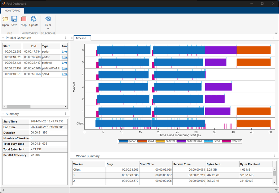
Pool Dashboard: Collect and analyze activity in parallel pools
Thread-Based Parallel Pool: Profile parallel code on thread workers
You can now use the mpiprofile command to profile
parallel code on workers of a thread-based parallel pool. For more information about
profiling your parallel code, see Profiling Parallel Code.
Cluster Profile Manager: Customize Threads profile
Manage the local machine Threads profile in the Cluster Profile
Manager. You can customize the preconfigured Threads profile by
editing the profile properties in the Cluster Profile Manager. You can also create
additional Threads profiles.
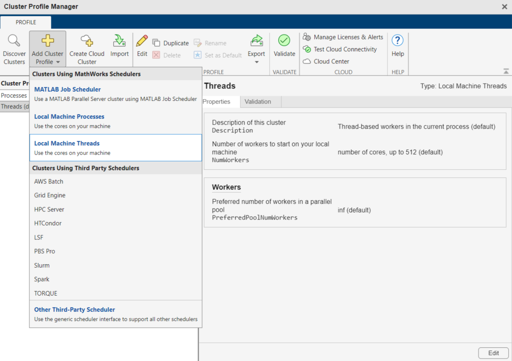
Cluster Profile Manager: Customize Threads profile
Profile Validation: Programmatically validate profile
Programmatically validate your profile using the parallel.validateProfile function. You can specify which validation
stages to run, set the number of workers to use, and write the validation results to
a file.
For example, you can validate the default profile.
parallel.validateProfile
Beginning validation for cluster profile 'Processes'
Cluster connection test (parcluster)
   Stage started at 15:35:45.
   Finished at 15:35:45.
..........................................................................PASSED

Job test (createJob)
   Stage started at 15:35:45.
   Finished at 15:36:04.
..........................................................................PASSED

SPMD job test (createCommunicatingJob)
   Stage started at 15:36:13.
   Job ran with 6 workers.
   Finished at 15:36:57.
..........................................................................PASSED

Pool job test (createCommunicatingJob)
   Stage started at 15:37:13.
   Job ran with 6 workers.
   Finished at 15:38:03.
..........................................................................PASSED

Parallel pool test (parpool)
   Stage started at 15:38:20.
   Connected to parallel pool with 6 workers.
   Parallel pool using the 'Processes' profile is shutting down.
   Parallel pool ran with 6 workers.
   Finished at 15:39:24.
..........................................................................PASSED

Finished cluster profile validation with status: PASSED
PollableDataQueue Objects: Enhanced functionality to simplify
data queue workflows
You can now create parallel.pool.PollableDataQueue
objects that allow the client or any worker in the pool to receive data.
The parallel.pool.PollableDataQueue function has a new
Destination name-value argument that enables you to specify
the destination behavior of the PollableDataQueue object. If you
want to send data to the client or any worker, set the
Destination argument to "any". Then any
worker with a copy of the PollableDataQueue object can poll it to
receive data. This new type of PollableDataQueue object simplifies
the process of sending data to workers during asynchronous
parfeval computations.
The PollableDataQueue object also has a new close object function to close a PollableDataQueue
object. Closing a PollableDataQueue object changes its new
isClosed property to true, which prevents you
from sending more data to the PollableDataQueue object.
For examples that show how to use the new type of
PollableDataQueue object, see Send Messages to Workers Using Pollable Data Queues and Transfer Data Between Workers Using Pollable Data Queues.
Parallel Pools: Partition pools from an existing parallel pool
Use the partition function to divide an existing parallel pool into subset
pools that allow you to utilize specific resources from the existing pool. Both the
partitioned pools and the input pool schedule work on the same underlying collection
of workers.
You can create pools that target specific workers to assign them specific roles or tasks. Additionally, you can create multiple pools to execute multiple parallel workflows simultaneously.
For example, you can partition a parallel pool to assign one worker to each cluster host in the pool.
hostPool = partition(pool,"MaxNumWorkersPerHost",1);Parallel Pools: Specify pool for parfor,
spmd, and Composite functions
The parfor, spmd, and Composite functions now accept
parallel.Pool objects as input
arguments. You can specify a pool object when you want to run computations on a pool
other than the pool the gcp function returns.
parpool Function: Add folders to workers search path
You can now add folders to the MATLAB search path of pool workers at the time of pool creation using the
AdditionalPaths name-value argument of the parpool function. This argument
ensures that pool workers look for code files, data files, or model files in the
correct locations.
GPU Functionality: Use functions with new and enhanced
gpuArray support
MATLAB
These MATLAB functions have new gpuArray support:
These MATLAB functions have enhanced gpuArray support:
min,max,sum,prod,ind2sub,rem,mod,power,realpow,mean,median,intmin,intmax,cummin,cummax,cumsum,cumprod— You can now use these functions with 64-bit integers.lsqminnorm— You can now specify a Tikhonov regularization factor.mean— You can now use the"native"output data type option.reshape— You can now reshape sparse GPU arrays.
For more information, see Run MATLAB Functions on a GPU. For a full list of MATLAB functions that accept GPU arrays, see Function List (GPU Arrays).
Statistics and Machine Learning Toolbox
These Statistics and Machine Learning Toolbox functions have new gpuArray support:
fitrkernel(Statistics and Machine Learning Toolbox),fitckernel(Statistics and Machine Learning Toolbox) — These functions and most of the object functions ofRegressionKernel(Statistics and Machine Learning Toolbox) andClassificationKernel(Statistics and Machine Learning Toolbox) models now support GPU array input arguments, allowing you to execute these functions on a GPU. The object functions that do not areincrementalLearner(Statistics and Machine Learning Toolbox),lime(Statistics and Machine Learning Toolbox), andshapley(Statistics and Machine Learning Toolbox).ocsvm(Statistics and Machine Learning Toolbox) — This function and theisanomaly(Statistics and Machine Learning Toolbox) object function ofOneClassSVM(Statistics and Machine Learning Toolbox) now support GPU array input arguments, enabling you to execute these functions on a GPU.
For a full list of Statistics and Machine Learning Toolbox functions that accept GPU arrays, see Function List (GPU Arrays) (Statistics and Machine Learning Toolbox).
Signal Processing Toolbox
These Signal Processing Toolbox functions have new gpuArray support:
envelope(Signal Processing Toolbox)envspectrum(Signal Processing Toolbox)fir1(Signal Processing Toolbox)
For a full list of Signal Processing Toolbox functions that accept GPU arrays, see Function List (GPU Arrays) (Signal Processing Toolbox).
Wavelet Toolbox
This Wavelet Toolbox function has new gpuArray support:
icwt(Wavelet Toolbox)
For a full list of Wavelet Toolbox functions that accept GPU arrays, see Function List (GPU Arrays) (Wavelet Toolbox).
5G Toolbox
These 5G Toolbox functions have new gpuArray support:
nrChannelEstimate(5G Toolbox)nrCRCEncode(5G Toolbox),nrCRCDecode(5G Toolbox)nrCodeBlockSegmentLDPC(5G Toolbox),nrCodeBlockDesegmentLDPC(5G Toolbox)nrLDPCEncode(5G Toolbox)nrRateMatchLDPC(5G Toolbox),nrRateRecoverLDPC(5G Toolbox)nrDLSCH(5G Toolbox),nrDLSCHDecoder(5G Toolbox)nrULSCH(5G Toolbox),nrULSCHDecoder(5G Toolbox)
For a full list of 5G Toolbox functions that accept GPU arrays, see Function List (GPU Arrays) (5G Toolbox).
Predictive Maintenance Toolbox
These Predictive Maintenance Toolbox™ functions have new gpuArray support:
distanceProfile(Predictive Maintenance Toolbox)findDiscord(Predictive Maintenance Toolbox)findMotif(Predictive Maintenance Toolbox)matrixProfile(Predictive Maintenance Toolbox)similarityDistance(Predictive Maintenance Toolbox)
For a full list of Predictive Maintenance Toolbox functions that accept GPU arrays, see Functions List (GPU Arrays) (Predictive Maintenance Toolbox).
Antenna Toolbox
These Antenna Toolbox™ functions have new gpuArray support:
raytrace(Antenna Toolbox),coverage(Antenna Toolbox),sinr(Antenna Toolbox),sigstrength(Antenna Toolbox),link(Antenna Toolbox),pathloss(Antenna Toolbox) — These functions support ray tracing analysis on a GPU when you specify aRayTracing(Antenna Toolbox) propagation model object as input and theUseGPUproperty of the object is"on"or"auto".
For a full list of Antenna Toolbox functions that accept GPU arrays, see Function List (GPU Arrays) (Antenna Toolbox).
Phased Array System Toolbox
These Phased Array System Toolbox™ functions have new gpuArray support:
For a full list of Phased Array System Toolbox functions that accept GPU arrays, see Function List (GPU Arrays) (Phased Array System Toolbox).
GPU Arrays: Reduce memory usage with single-precision sparse GPU arrays
You can now create and use single-precision sparse GPU arrays. Sparse matrices provide efficient storage of data that has a large percentage of zeros and reduce computation time by eliminating operations on zero elements. Single-precision sparse GPU arrays allow you to reduce memory usage and accelerate calculations by taking advantage of your GPU's single-precision floating-point units (FPUs).
You can convert a sparse gpuArray to a single-precision array
using the single function, or you can create
a sparse, single-precision gpuArray directly by specifying the
typename argument as "single" when you
create a sparse gpuArray. For example, this code creates a
1000-by-1000 random, single-precision, sparse gpuArray with density
0.1.
R = gpuArray.sprand(1000,1000,0.1,"single");For more information, see Work with Sparse Arrays on a GPU.
GPU arrayfun: Support for like syntax of
intmin, intmax,
realmin, and realmax
You can now use the intmin, intmax, realmin, and realmax functions and specify a
prototype array using the like syntax in functions you apply
using the arrayfun function.
For example, this function uses intmin and
intmax to determine whether elements of integer
gpuArray
x are saturated.
function saturated = findSaturated(x)
saturated = (x == intmin(like=x)) | (x == intmax(like=x));
end

% Generate random integer gpuArray that includes saturated values.
x = randi([-200 200],1e6,1,"int8","gpuArray");

% Find saturated values.
saturated = arrayfun(@findSaturated,x);
GPU Workflow Examples: New and updated GPU computing examples
This updated example shows how to measure key performance characteristics of your GPU hardware:
This new example shows how to use GPU computing to accelerate data preprocessing and deep learning for predictive maintenance workflows:
Accelerate Fault Diagnosis Using GPU Data Preprocessing and Deep Learning (Predictive Maintenance Toolbox)
These new and updated examples show how to use GPU computing to accelerate 5G simulations:
Accelerate 5G Simulation Using GPU (5G Toolbox)
NR PDSCH Throughput (5G Toolbox)
This new example shows how to perform accelerated ray tracing analysis using a GPU:
Accelerate Ray Tracing Analysis Using GPU (Antenna Toolbox)
GPU arrayfun: Support for using P-code files in compiled
standalone applications
You can now call the arrayfun function inside P-code
files or use arrayfun to evaluate functions obfuscated as a
P-code file in standalone applications compiled using MATLAB
Compiler™.
For more information about packaging a MATLAB function into a standalone application, see Create Standalone Application from MATLAB (MATLAB Compiler).
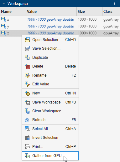
GPU Arrays: Gather GPU arrays interactively from workspace
You can now gather gpuArray objects by right-clicking the
variable in the workspace, and then selecting Gather from
GPU. This action is equivalent to calling the gather function on a
gpuArray object.
GPU Statistics Functions: Improved performance for mean,
movmean, movstd, and
movvar
Mean
These syntaxes of the mean function show improved
performance on a GPU:
M = mean(A)M = mean(A,"all")M = mean(A,dim), wheredimis a scalar double
Improvements are greater when you operate on smaller arrays. For example, computing the mean of a matrix in this code is about 2.4x faster than in the previous release.
function timeMean

% Reset GPU device.
reset(gpuDevice)

% Create random gpuArray data.
X = rand(200,"gpuArray");

% Time mean function.
f = @() mean(X,"all");
gputimeit(f)

end
The approximate execution times are:
R2024b: 63.9 microseconds
R2025a: 26.9 microseconds
The code was timed on a Windows 10, Intel
Xeon W-2133 @ 3.60 GHz test system with an NVIDIA RTX A5000 GPU by calling the timeMean
function.
Moving Mean, Standard Deviation, and Variance
The movmean, movstd, and movvar functions show improved
performance on a GPU. For example, computing the five-point centered moving
average of a matrix in this code is about 1.6x faster than in the previous
release.
function timeMovmean

% Reset GPU device.
reset(gpuDevice)

% Create random gpuArray data.
X = rand(1e4,"gpuArray");

% Time movmean function.
f = @() movmean(X,5);
gputimeit(f)

end
The approximate execution times are:
R2024b: 14.8 milliseconds
R2025a: 9.2 milliseconds
The code was timed on a Windows 10, Intel
Xeon W-2133 @ 3.60 GHz test system with an NVIDIA RTX A5000 GPU by calling the timeMovmean
function.
GPU histcounts: Improved performance
The histcounts function shows improved
performance on a GPU. Improvements are greater when you operate on smaller arrays.
For example, partitioning values into 21 bins and returning the bin counts and bin
edges in the following code is about 1.7x faster than in the previous
release:
function timeHistcounts

% Reset GPU device.
reset(gpuDevice)

% Create random input data.
X = rand(1000,"gpuArray");

% Time histcounts function.
f = @() histcounts(X,21);
gputimeit(f,2)

end
The approximate execution times are:
R2024b: 1.2 milliseconds
R2025a: 0.7 milliseconds
The code was timed on a Windows 10, Intel
Xeon W-2133 @ 3.60 GHz test system with an NVIDIA RTX A5000 GPU by calling the timeHistcounts
function.
Tall Arrays: Support for isuniform
The isuniform function has new tall array support. For more information,
see Tall Arrays for Out-of-Memory Data.
Distributed Arrays: Reduce memory usage with single-precision sparse distributed arrays
You can now create and use single-precision sparse distributed and codistributed arrays. Sparse matrices provide efficient storage of data that has a large percentage of zeros and reduce computation time by eliminating operations on zero elements. Single-precision sparse distributed and codistributed arrays allow you to reduce memory usage. You can create single-precision sparse distributed and codistributed arrays using these functions:
By default, these functions create a double-precision sparse distributed or
codistributed array. To create single-precision sparse distributed or codistributed
arrays, specify the new typename argument as
"single". For example, this code creates a 50-by-100
single-precision sparse distributed array with density
0.1.
distributed.sprandn(50,100,0.1,"single")You can also create single-precision sparse distributed or codistributed arrays by
providing single-precision distributed or codistributed arrays to the
sparse function.
Distributed Arrays: Use functions with new and enhanced distributed array support
These functions have new and enhanced distributed array support:
mean— You can now use the"native"output data type option.
For more information, see Run MATLAB Functions with Distributed Arrays.
Parallel Workflows: New and Updated Examples and Topics
Use these new examples to progress with parallel computing:
Try Parallel Computing Methods — This new example shows how to accelerate your MATLAB code using parallel computing.
Optimize
parfor-Loops with Pool Dashboard — This new example shows how to use the Pool Dashboard to understand how workers execute yourparfor-loop and how you can optimize it.Perform Data Acquisition and Processing on Pool Workers — This new example shows how to use
PollableDataQueueobjects to control the movement of data between workers in a parallel data acquisition and processing pipeline.Control Hardware and Acquire Data in Parallel — This new example shows how to use the
parfevalfunction andPollableDataQueueobjects to simultaneously control hardware and perform data acquisition using parallel workers.
Support for Intel MPI
Parallel computing products now ship with Intel MPI Library for use on Linux for third-party schedulers.
To use Intel MPI, set the MPIImplementation additional
property for your third-party cluster profile or object to
"IntelMPI". To learn more about setting additional
properties, see Set Additional Properties (MATLAB Parallel Server).
Support for MPICH: Upgrade to MPICH 4.2.2
Parallel computing products now ship with MPICH version 4.2.2 for use on Linux for third-party schedulers.
Functionality being removed or changed
MPICH2 is removed
Errors
Starting in R2025a, parallel computing products no longer ship with MPICH2.
Support for Volta GPUs will be removed
Warns
Support for Volta architecture GPUs with compute capability 7.0 will be removed in a future release. At that time, GPU computing in MATLAB will require a GPU device with compute capability 7.5 or greater.
In R2025a, Volta architecture GPUs are still supported. MATLAB issues a warning the first time you use a Volta GPU.
For more information about supported GPU devices, see GPU Computing Requirements.
parfor-Loops: Use colon-vector indexing expressions with
sliced variables
You can now use colon-vector expressions to index sliced input and output
variables in parfor-loop statements.
Colon-vector indexing expressions allow you to use more natural forms of indexing
for parfor output variables, eliminating the need for nested
for-loops. The colon-vector indexing expression must be in
the form j:k or j:k:l.
For example, to assign values to columns 3 to 7 of the output variable
out, use the colon-vector 3:7 as a
subscript when you index the sliced
variable.
out = zeros(10);
parfor i = 1:10
    out(i,3:7) = rand(1,5);
end
Starting in R2024b, indexing a sliced variable with a colon-vector expression no longer throws an error. For more information, see parfor no longer errors when you index sliced variables with colon-vector expressions.
Thread-Based Environment: Use Image Processing Toolbox functionality on thread workers
These Image Processing Toolbox functions can now run in a thread-based environment:
dicomanon(Image Processing Toolbox)dicomCollection(Image Processing Toolbox)dicomContours(Image Processing Toolbox) and its functionsaddContour(Image Processing Toolbox),convertToInfo(Image Processing Toolbox),createMask(Image Processing Toolbox), anddeleteContour(Image Processing Toolbox)dicomdict(Image Processing Toolbox)dicomdisp(Image Processing Toolbox)dicomfind(Image Processing Toolbox)dicominfo(Image Processing Toolbox)dicomlookup(Image Processing Toolbox)dicomread(Image Processing Toolbox)dicomreadVolume(Image Processing Toolbox)dicomupdate(Image Processing Toolbox)dicomuid(Image Processing Toolbox)dicomwrite(Image Processing Toolbox)images.dicom.decodeUID(Image Processing Toolbox)images.dicom.parseDICOMDIR(Image Processing Toolbox)
For more information, see Run MATLAB Functions in Thread-Based Environment.
GPU Validation: Verify GPU device setup
Use the validateGPU function to verify that MATLAB can use your GPU and to diagnose issues.
For example, you can validate the currently selected GPU. If no GPU device is selected, then the function validates the default device.
validateGPU
# Beginning GPU validation
# Performing system validation
#    CUDA-supported platform .................................................PASSED
#    CUDA-enabled graphics driver exists .....................................PASSED
#        Version: 537.70
#    CUDA-enabled graphics driver load .......................................PASSED
#    CUDA environment variables ..............................................PASSED
#    CUDA device count .......................................................PASSED
#        Found 2 devices.
#    GPU libraries load ......................................................PASSED
#
# Performing device validation for device index 1
#    Device exists ...........................................................PASSED
#        NVIDIA RTX A5000
#    Device supported ........................................................PASSED
#    Device available ........................................................PASSED
#        Device is in 'Default' compute mode.
#    Device selectable .......................................................PASSED
#    Device memory allocation ................................................PASSED
#    Device kernel launch ....................................................PASSED
#
# Finished GPU validation with no failures.
GPU Device: New device properties and updated display
Use the gpuDevice function to inspect
these new properties of your GPU device:
LastAccessed— the date and time the device was last accessed by the current MATLAB session.SingleDoubleRatio— the ratio of single- to double-precision floating point units (FPUs) on the device.
Creating or querying a GPUDevice object now displays only the
Name, Index,
ComputeCapability, DriverModel,
TotalMemory, AvailableMemory,
DeviceAvailable, and DeviceSelected
properties. To view all of the properties of a device, create or query a
GPUDevice object without suppressing output and click the
Show all properties link.
D = gpuDevice
D =

  CUDADevice with properties:

                 Name: 'NVIDIA RTX A5000'
                Index: 1 (of 2)
    ComputeCapability: '8.6'
          DriverModel: 'TCC'
          TotalMemory: 25544294400 (25.54 GB)
      AvailableMemory: 25120866304 (25.12 GB)
      DeviceAvailable: true
       DeviceSelected: true

  Show all properties.
The SupportsDouble,
GPUOverlapsTransfers, and CanMapHostMemory
properties are no longer displayed but you can still query these properties using
dot notation. There are no plans to remove these properties.
GPU Functionality: Use functions with new and enhanced
gpuArray support
MATLAB
These MATLAB functions have new gpuArray support:
These MATLAB functions have enhanced gpuArray support:
bicg,bicgstab,cgs,gmres,lsqr,pcg,qmr,tfqmr— When you solve sparse linear systems, you can now provide a lower triangular matrix and an upper triangular matrix as preconditioner matrices. For more information, see GPU Sparse Solvers: Use triangular preconditioner matrices to solve sparse linear systems.cumsum— You can now use thenanflagargument to specify whether the function includes missing values when calculating the cumulative sums.imresize— You can now resize images or arrays of images with more than 227 elements.plus,minus,times,rdivide,ldivide,median— You can now use these functions with 64-bit integers.
For more information, see Run MATLAB Functions on a GPU.
Statistics and Machine Learning Toolbox
These Statistics and Machine Learning Toolbox functions have new and enhanced gpuArray support:
fitcecoc(Statistics and Machine Learning Toolbox) — You can now specify linear and ensemble learners when you create aClassificationECOC(Statistics and Machine Learning Toolbox),CompactClassificationECOC(Statistics and Machine Learning Toolbox),ClassificationPartitionedECOC(Statistics and Machine Learning Toolbox), orClassificationPartitionedLinearECOC(Statistics and Machine Learning Toolbox) model object by passing agpuArrayinput tofitcecoc.fitrnet(Statistics and Machine Learning Toolbox),fitcnet(Statistics and Machine Learning Toolbox) — These functions and the object functions of the modelsRegressionNeuralNetwork(Statistics and Machine Learning Toolbox),CompactRegressionNeuralNetwork(Statistics and Machine Learning Toolbox),RegressionPartitionedNeuralNetwork(Statistics and Machine Learning Toolbox),ClassificationNeuralNetwork(Statistics and Machine Learning Toolbox), andCompactClassificationNeuralNetwork(Statistics and Machine Learning Toolbox) now accept GPU array input arguments, enabling you to execute these functions on a GPU.
For a full list of Statistics and Machine Learning Toolbox functions that accept GPU arrays, see Function List (GPU Arrays) (Statistics and Machine Learning Toolbox).
Signal Processing Toolbox
These Signal Processing Toolbox functions and objects have new and enhanced
gpuArray support:
hht(Signal Processing Toolbox)tfridge(Signal Processing Toolbox)signalDatastore(Signal Processing Toolbox) — You can now return data on the GPU by setting theOutputEnvironmentproperty to"gpu".signalTimeFrequencyFeatureExtractor(Signal Processing Toolbox)
For a full list of Signal Processing Toolbox functions that accept GPU arrays, see Function List (GPU Arrays) (Signal Processing Toolbox).
Wavelet Toolbox
This Wavelet Toolbox function has new gpuArray support:
modwptdetails(Wavelet Toolbox)
For a full list of Wavelet Toolbox functions that accept GPU arrays, see Function List (GPU Arrays) (Wavelet Toolbox).
Communications Toolbox
These Communications Toolbox functions have new and enhanced gpuArray support:
ldpcEncode(Communications Toolbox)pskdemod(Communications Toolbox)pskmod(Communications Toolbox)
For a full list of Communications Toolbox functions that accept GPU arrays, see Function List (GPU Arrays) (Communications Toolbox).
5G Toolbox
These 5G Toolbox functions have new and enhanced gpuArray support:
nrCDLChannel(5G Toolbox)nrPDSCH(5G Toolbox)nrPDSCHDecode(5G Toolbox)nrPUSCH(5G Toolbox)nrPUSCHDecode(5G Toolbox)nrPUSCHScramble(5G Toolbox)nrPerfectChannelEstimate(5G Toolbox)nrPerfectTimingEstimate(5G Toolbox)nrExtractResources(5G Toolbox)
For a full list of 5G Toolbox functions that accept GPU arrays, see Function List (GPU Arrays) (5G Toolbox).
Image Processing Toolbox
This Image Processing Toolbox function has new gpuArray support:
montage(Image Processing Toolbox)
For a full list of Image Processing Toolbox functions that accept GPU arrays, see Function List (GPU Arrays) (Image Processing Toolbox).
GPU Sparse Solvers: Use triangular preconditioner matrices to solve sparse linear systems
You can now provide a lower triangular matrix and an upper triangular matrix as preconditioner matrices when you solve sparse linear systems on a GPU using these functions:
Using lower triangular and upper triangular preconditioner matrices can significantly improve convergence of the algorithm.
% Create sparse coefficient matrix.
gridDimension = 1024;
A = delsq(numgrid("A",gridDimension));

% Create right-hand side vector.
b = zeros(size(A,1),1);
b(1000) = 1;

% Use incomplete LU factorization to create lower and upper triangular
% preconditioner matrices.
options.type = "ilutp";
options.droptol = 1e-6;
options.thresh = 0;
[L,U] = ilu(A,options);

% Solve system of linear equations with preconditioner matrices.
A = gpuArray(A);
tol = 1e-12;
maxit = 20;
x = gmres(A,b,[],tol,maxit,L,U);
GPU arrayfun: Support for P-code files and functions defined
in class definition files
You can now use P-code files with arrayfun. You can:
Use
arrayfunto evaluate a function obfuscated as a P-code file.Call
arrayfuninside a P-code file.Use
arrayfunwhen the function it applies contains a call to a function obfuscated as a P-code file.
For more information about P-code files, see Create a Content-Obscured File with P-Code.
You can also call arrayfun in a class method to evaluate
functions defined in the class definition file (a file with a .m
extension that contains the classdef keyword).
For example, this class contains a method, output, that uses
arrayfun to evaluate a local function,
localFun.
classdef TestClass
    methods
        function output = func(obj,x)
            output = arrayfun(@localFun,x);
        end
    end
end

function output = localFun(x)
output = x.*x;
end
For more information about defining classes in MATLAB, see Creating a Simple Class.
GPU mldivide: Improved performance for overdetermined
systems
The mldivide function
(\) shows improved performance when solving linear systems on
a GPU when input matrix A has more rows than columns (the system
is overdetermined) and has at least 5000 elements. For example, in the following
code, solving a sparse linear system with an 80-by-81 input matrix is about 1.8x
faster than in the previous release:
function timeMldivide

% Create rectangular matrix and column vector.
n = 80;
A = rand(n+1,n,"gpuArray");
b = rand(n+1,1,"gpuArray");

% Time mldivide.
gputimeit(@() A\b)

end
The approximate execution times are:
R2024a: 4.6 milliseconds
R2024b: 2.5 milliseconds
The code was timed on a Windows 10, Intel
Xeon W-2133 @ 3.60 GHz test system with an NVIDIA RTX A5000 GPU by calling the timeMldivide
function.
GPU Sparse mldivide: Improved performance for triangular
matrices
The mldivide function
(\) shows improved performance and reduced memory usage on a
GPU when solving sparse linear systems with a triangular input matrix
A. For example, in the following code, solving a sparse
linear system with a 271201-by-271201 input matrix is about 1800x faster than in the
previous release:
function timeSparseMldivide

% Create sparse triangular matrix.
n = 300;
A = gallery("wathen",n,n);
A = tril(A);
A = gpuArray(A);

% Create dense vector.
b = ones(size(A,1),1,"gpuArray");

% Time mldivide.
gputimeit(@() A\b)

end
The approximate execution times are:
R2024a: 36.3 s
R2024b: 0.02 s
The code was timed on a Windows 10, Intel
Xeon W-2133 @ 3.60 GHz test system with an NVIDIA RTX A5000 GPU by calling the timeSparseMldivide
function.
GPU Cholesky Factorization: Improved performance
The chol function shows improved
performance on a GPU when factorizing matrices that are at least 600-by-600. For
example, factorizing the matrix in the following code is about 1.4x faster than in
the previous release:
function timeChol

% Create symmetric positive definite matrix.
n = 1000;
A = rand(n,"gpuArray");
SPD = A'*A;

% Time Cholesky factorization.
gputimeit(@() chol(SPD))

end
The approximate execution times are:
R2024a: 59 milliseconds
R2024b: 41 milliseconds
The code was timed on a Windows 10, Intel
Xeon W-2133 @ 3.60 GHz test system with an NVIDIA RTX A5000 GPU by calling the timeChol
function.
GPU LU Factorization: Improved performance of two-output syntax
The lu function shows improved
performance on a GPU when returning two outputs and factorizing matrices that are at
least 140-by-140. For example, factorizing the matrix in the following code is about
2.4x faster than in the previous release:
function timeLU

% Create symmetric positive definite matrix.
n = 300;
A = rand(n,"gpuArray");
SPD = A'*A;

% Time LU factorization.
gputimeit(@() lu(SPD),2)

end
The approximate execution times are:
R2024a: 31 milliseconds
R2024b: 13 milliseconds
The code was timed on a Windows 10, Intel
Xeon W-2133 @ 3.60 GHz test system with an NVIDIA RTX A5000 GPU by calling the timeLU
function.
GPU arrayfun: Improved performance when parent workspace
variable changes size
The arrayfun function shows improved
performance on a GPU when the function applied by arrayfun uses
a variable in the workspace of a parent function and that variable changes size. If
the number of dimensions of the variable in the workspace of the parent function
changes, then there is no performance improvement. For example, calling
arrayfun several times in the following code is about 11.2x
faster than in the previous release:
function timeArrayfun

% Reset GPU to clear previously compiled functions.
gpuDevice([]);
gpu = gpuDevice;
wait(gpu)

% Create array of sizes.
size = 10:1:1000;

% Time arrayfun call while changing the size of array upLevel.
tic
for idx = 1:numel(size)
    upLevel = rand(size(idx),"gpuArray");
    randomIndex = randi(numel(upLevel),10,"gpuArray");

    out = arrayfun(@accessUplevel,randomIndex);
end
toc

    function out = accessUplevel(randomIndex)
        % Define function called by arrayfun that accesses variable in
        % parent workspace.
        out = upLevel(randomIndex);
    end

end
The approximate execution times are:
R2024a: 4.71 s
R2024b: 0.42 s
The code was timed on a Windows 10, Intel
Xeon W-2133 @ 3.60 GHz test system with an NVIDIA RTX A5000 GPU by calling the timeArrayfun
function.
Job Properties: Determine the storage size (in bytes) of jobs
You can now determine the number of bytes the data for your job occupies in the
job storage location. The data includes task input and output arguments, attached
files, and entries in the job's FileStore and ValueStore objects.
To access the storage size (in bytes) of your job, query the
StorageBytes property of the parallel.Job object.
job = batch(@rand,1,{5});
job.StorageBytes
ans = 9425
You can also view the storage size of your job in the Job Monitor.
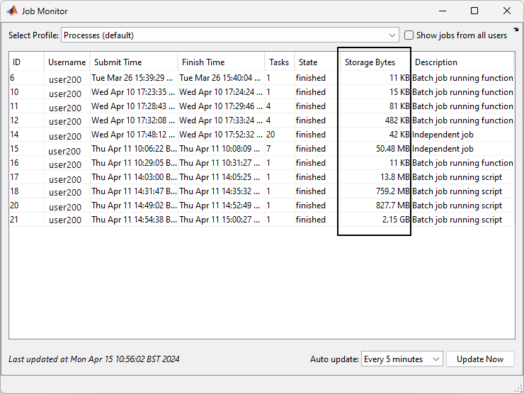
Job Properties: Determine the storage size (in bytes) of jobs
Cluster Administration: Export cluster monitoring metrics for integration with Prometheus and Grafana
Set up your MATLAB Job Scheduler to export cluster monitoring metrics such as cluster status, worker utilization, and licenses in use. Use these metrics to monitor the health of the MATLAB Job Scheduler cluster, diagnose issues, and optimize performance.
You can gather the exported metrics with a cluster monitoring system such as Prometheus® and visualize them in a preconfigured Grafana® dashboard. This setup allows for live cluster monitoring and alerts. For more information, see Configure Metrics for MATLAB Job Scheduler (MATLAB Parallel Server).
Gather In-Memory Arrays: Improved performance
The gather function shows improved
performance when the input is not a gpuArray,
distributed array, or tall array. For
example, gathering the data in the following code is about 9x faster than in the
previous release:
function timeGather

% Create in-memory data.
x = 1;

% Time gather operations.
n = 1e7;
tic
for idx = 1:n
    y = gather(x);
end
toc/n

end
The approximate execution times are:
R2024a: 0.51 microseconds
R2024b: 0.06 microseconds
The code was timed on a Windows 10, Intel
Xeon W-2133 @ 3.60 GHz test system by calling the
timeGather function.
Distributed Arrays: Use functions with new distributed array support
These functions have new and enhanced distributed array support:
contains,count,endsWith,erase,eraseBetween,extractAfter,extractBefore,extractBetween,insertAfter,insertBefore,matches,replace,replaceBetween,startsWith,strfind— You can now use these functions withpatternobjects.
For more information, see Run MATLAB Functions with Distributed Arrays.
Tall Arrays: Use functions with new and enhanced tall array support
These functions have new and enhanced tall array support:
contains,count,endsWith,erase,eraseBetween,extractAfter,extractBefore,extractBetween,insertAfter,insertBefore,matches,replace,replaceBetween,split,startsWith,strfind— You can now use these functions withpatternobjects.
For more information, see Tall Arrays for Out-of-Memory Data.
Signal Processing: New examples
These new examples show how to accelerate signal feature extraction and classification:
Accelerate Signal Feature Extraction and Classification Using a Parallel Pool of Workers (Signal Processing Toolbox)
Accelerate Signal Feature Extraction and Classification Using a GPU (Signal Processing Toolbox)
Support for MPICH: Upgrade to MPICH 4.1.2
Parallel computing products now ship with MPICH 4.1.2 for use on Linux for third-party schedulers.
Functionality being removed or changed
parfor no longer errors when you index sliced variables
with colon-vector expressions
Behavior change
In R2024b, you can index sliced variables in parfor-loop
statements with colon-vector indexing expressions. Before R2024b, indexing
sliced variables with colon-vector expressions results in an error. If you have
code that relies on this behavior, update your code to avoid compatibility
issues.
Support for Pascal GPUs will be removed
Warns
Support for Pascal architecture GPUs with compute capability 6.0 to 6.2 will be removed in a future release. At that time, GPU computing in MATLAB will require a GPU device with compute capability 7.0 or greater.
In R2024b, Pascal architecture GPUs are still supported. MATLAB issues a warning the first time you use a Pascal GPU.
For more information about supported GPU devices, see GPU Computing Requirements.
Improved Scalability: Support for parallel pools with up to 2000 workers
Parallel Computing Toolbox now supports parallel pools with up to 2000 workers. To learn about parallel pools, see Run Code on Parallel Pools.
Thread-Based Parallel Pool: Specify maximum number of thread workers in
parfor-loop
You can now specify the maximum number of workers when executing parfor-loops on a thread-based
parallel pool.
For example, this code starts a pool with 6 thread workers and runs the body of a
parfor-loop on a maximum of 2 thread
workers.
parpool("Threads",6);
parfor (i=1:6,2)
disp(i)
end
Starting in R2024a, specifying the maximum number of thread workers in a
parfor-loop no longer throws an error. For more
information, see parfor no longer errors when you specify maximum number of thread workers in parfor-loop.
Thread-Based Environment: Use new functionality on thread workers
These MATLAB functions now have thread-based support:
For more information, see Run MATLAB Functions in Thread-Based Environment.
GPU Functionality: Use functions with new and enhanced
gpuArray support
MATLAB
These MATLAB functions have new and enhanced gpuArray support:
bitget— You can now use this function with unsigned integers and 64-bit integers.bitset— You can now use this function with unsigned integers and 64-bit integers.sound— This function now accepts GPU arrays but does not run on a GPU.soundsc— This function now accepts GPU arrays but does not run on a GPU.subsref— You can now reference entire rows or columns of sparse GPU arrays by index.
For more information, see Run MATLAB Functions on a GPU.
Statistics and Machine Learning Toolbox
These Statistics and Machine Learning Toolbox functions have new gpuArray support:
The
fitrlinear(Statistics and Machine Learning Toolbox) andfitclinear(Statistics and Machine Learning Toolbox) functions accept GPU array input arguments and can execute on a GPU.Most object functions of the models
RegressionLinear(Statistics and Machine Learning Toolbox),RegressionPartitionedLinear(Statistics and Machine Learning Toolbox),ClassificationLinear(Statistics and Machine Learning Toolbox), andClassificationPartitionedLinear(Statistics and Machine Learning Toolbox) now support GPU array input arguments and can execute on a GPU. The following functions do not support GPU array input arguments:RegressionLinear—incrementalLearner,lime,shapley, andupdateClassificationLinear—incrementalLearner,lime,shapley, andupdate
geomean(Statistics and Machine Learning Toolbox),harmmean(Statistics and Machine Learning Toolbox),trimmean(Statistics and Machine Learning Toolbox) — You can now use theallandvecdiminput arguments.
For a full list of Statistics and Machine Learning Toolbox functions with GPU functionality, see Functions with gpuArray
support (Statistics and Machine Learning Toolbox).
Communications Toolbox
These Communications Toolbox system objects and functions have new gpuArray support:
comm.MIMOChannel(Communications Toolbox)comm.ChannelFilter(Communications Toolbox)ofdmChannelResponse(Communications Toolbox)genqammod(Communications Toolbox)bit2int(Communications Toolbox)int2bit(Communications Toolbox)biterr(Communications Toolbox)
For a full list of Communications Toolbox functions with GPU functionality, see Functions with gpuArray
support (Communications Toolbox).
5G Toolbox
These 5G Toolbox functions have new gpuArray support:
nrOFDMModulate(5G Toolbox)nrOFDMDemodulate(5G Toolbox)nrSymbolModulate(5G Toolbox)nrSymbolDemodulate(5G Toolbox)nrLDPCDecode(5G Toolbox)nrEqualizeMMSE(5G Toolbox)
For a full list of 5G Toolbox functions with GPU functionality, see Functions with gpuArray
support (5G Toolbox).
Audio Toolbox
This Audio Toolbox™ object has new gpuArray support:
audioDatastore(Audio Toolbox) — You can now return data on the GPU by setting theOutputEnvironmentproperty to"gpu".
For a full list of Audio Toolbox functions with GPU functionality, see Functions with gpuArray
support (Audio Toolbox).
Wavelet Toolbox
This Wavelet Toolbox function has new gpuArray support:
wsst(Wavelet Toolbox)
For a full list of Wavelet Toolbox functions with GPU functionality, see Functions with gpuArray
support (Wavelet Toolbox).
GPU arrayfun: Support for cell array case expressions in
switch, case,
otherwise
Use a cell array as the case expression to compare the switch expression against
multiple values with switch, case, otherwise within the
function you apply using arrayfun. For example, you can use
case {x1,y1} to execute the corresponding code if the
switch expression matches at least one of
x1 and y1.
GPU Device: Identify GPUs using their UUIDs
Inspect the universally unique identifier (UUID) of your GPU using the
UUID property of a GPUDevice object. You
can use the UUID to distinguish otherwise identical GPUs.
For example, you can inspect the UUID of four GPUs using the gpuDeviceTable function.
gpuDeviceTable(["Index","Name","UUID"])
    Index           Name                              UUID
    _____    __________________    __________________________________________

      1      "NVIDIA RTX A5000"    "GPU-957b509e-322a-ae88-59c8-b7435d0f98f4"
      2      "NVIDIA RTX A5000"    "GPU-6f3ad2c0-5ea1-b1a2-1dca-cd756d10dbc0"
      3      "NVIDIA RTX A5000"    "GPU-41c24f34-c915-919b-0bb3-20d07117e0ec"
      4      "NVIDIA RTX A5000"    "GPU-23ab01ce-2f42-2d0c-0f6b-db7ac8c10867"
Alternatively, you can select a GPU using the gpuDevice function and query its
UUID.
D = gpuDevice;
D.UUID
'GPU-957b509e-28ca-ae88-59c8-b7435d0f98f4'
Cluster Administration: Access MATLAB Job Scheduler job history
You can now access job history information about MATLAB Parallel Server use on your MATLAB Job Scheduler. This information allows you to audit cluster usage and gain insight into cluster usage patterns based on job type, MATLAB version, and task duration.
For more information, see Manage and Access MATLAB Job Scheduler Cluster Job History (MATLAB Parallel Server).
MATLAB Parallel Server in Spark: Enhanced support for Spark clusters
This release introduces enhanced support for Spark™ based clusters integrated with MATLAB Parallel Server.
You can now create and validate cluster profiles for Spark based clusters integrated with MATLAB Parallel Server. Cluster profiles allow you to define properties for the Spark cluster object using the Cluster Profile Manager or from the command line. You can also export and share the cluster profile with other MATLAB users to connect to the cluster. For more details about creating Spark cluster profiles, see Configure for Spark Clusters (MATLAB Parallel Server).
parallel.cluster.Spark cluster objects now have support for
several Common Job Scheduler properties and object functions. For more details, see
parallel.cluster.Spark.
Distributed Arrays: Use functions with new distributed array support
These functions have new and enhanced distributed array support:
For more information, see Run MATLAB Functions with Distributed Arrays.
Workflow Examples: New and updated examples and topics
This new example shows how to use datastores to transform large raw data into a state ready for future analysis and save to Parquet files using parallel workers:
These new examples show how to accelerate your code using a GPU:
Accelerate Audio Machine Learning Workflows Using a GPU (Audio Toolbox)
Accelerate MIMO-OFDM Link Simulation Using GPU (Communications Toolbox)
These new topics and examples show different approaches for scaling up parallel code to accommodate large-scale computations on HPC clusters:
This updated example shows how to solve a simple optimization problem using
parfeval:
GPU Support: Upgrade to CUDA 12.2
GPU computing in MATLAB now uses CUDA 12.2. You can use new CUDA features when you write custom CUDA code for running in MATLAB via mexcuda or parallel.gpu.CUDAKernel.
Kepler architecture GPUs are no longer supported. For more information, see Support for Kepler architecture GPUs is removed.
The supported version of the CUDA toolkit is now version 12.2. For more information, see Change to supported CUDA Toolkit.
Parallel Batch Jobs: Disable SPMD support for parallel pools in batch jobs
You can now configure the parallel pools in batch jobs offloaded to local or
MATLAB Job Scheduler clusters to run without single-program multiple-data
(SPMD) support. This settings allows parallel pools to keep running even if workers
abort during parfor execution.
To disable SPMD support, set the SpmdEnabled name-value
argument to false in the call to the batch or createCommunicatingJob function. For
example, this code offloads a job that runs the myFunction
function on a parallel pool without SPMD
support.
j = batch(@myFunction,1,{x,y},Pool=4,SpmdEnabled=false)Third-Party Cluster Schedulers: Built-in integrations now align with plugin scripts
When you integrate MATLAB with your third-party scheduler using a built-in cluster profile, MATLAB now derives the built-in cluster profile from the generic plugin scripts published on GitHub. This change allows you to access the range of features available with the plugin scripts and customize how MATLAB interfaces with your scheduler setup.
Third-Party Cluster Schedulers: Use integrations for AWS Batch, Grid Engine, and HTCondor schedulers
The Add Cluster Profile button in the Cluster Profile Manager now includes options to create cluster profiles for AWS Batch, Grid Engine, and HTCondor scheduler clusters. When you select one of these options, the software creates a scheduler specific default profile which you can modify as needed.
Sparse Matrix Products: Improved performance on GPU
Computing the product of some sparse matrices on the GPU shows improved performance. The amount of speedup depends on the sparsity pattern of the matrix. For example, in the following code, computing the product of two sparse matrices is about 6x faster than in the previous release:
function timeSparseMatrixProduct

% Create sparse matrix.
A = gpuArray(gallery("neumann",4000000));

% Time matrix product.
gputimeit(@() A*A)

end
The approximate execution times are:
R2023b: 0.06 s
R2024a: 0.01 s
The code was timed on a Windows 10, Intel
Xeon W-2133 @ 3.60 GHz test system with an NVIDIA RTX A5000 GPU by calling the
timeSparseMatrixProduct function.
Preconditioned Sparse Solvers: Improved performance using preconditioned iterative solvers on GPU
Solving large sparse linear systems using preconditioned iterative solvers on the
GPU shows improved performance. The amount of speedup depends on the sparsity
pattern of the matrices. For example, in the following code, solving a sparse linear
system with a 752001-by-752001 coefficient matrix using the bicg function is about 33x faster
than in the previous release:
function timePreconditionedSolver

% Create large sparse matrix.
A = gpuArray(gallery("wathen",500,500));

% Create a random right-hand side matrix.
actualSolution = rand(size(A,1),1);
b = A*actualSolution;

% Create preconditioner matrix.
k = 3;
M = tril(triu(A,-k),k);

% Time solver.
maxNumberOfIterations = 100;
gputimeit(@() bicg(A,b,[],maxNumberOfIterations,M))

end
The approximate execution times are:
R2023b: 26.8 s
R2024a: 0.8 s
The code was timed on a Windows 10, Intel
Xeon W-2133 @ 3.60 GHz test system with an NVIDIA RTX A5000 GPU by calling the
timePreconditionedSolver function.
Functionality being removed or changed
Support for Kepler architecture GPUs is removed
Errors
Starting in R2024a, Kepler architecture GPUs are no longer supported and the
range of compute capabilities supported is 5.0 to
9.x.
For more information, see GPU Computing Requirements.
Change to supported CUDA Toolkit
Errors
Starting in R2024a, CUDA Toolkit version 11.8 is no longer supported. To create parallel.gpu.CUDAKernel objects
using libraries that are not installed with MATLAB or if you have previously installed the CUDA Toolkit, install CUDA Toolkit version 12.2 instead.
For more information, see Install CUDA Toolkit (Optional).
parfor no longer errors when you specify maximum number
of thread workers in parfor-loop
Behavior change
In R2024a, you can specify the maximum number of thread workers to execute
your parfor-loop. Before R2024a, specifying the maximum
number of thread workers to execute a parfor-loop results
in an error. If you have code that relies on this behavior, update your code to
avoid compatibility issues. If you do not specify the maximum number of workers
for a parfor-loop, MATLAB uses as many workers as are available in your parallel pool, as in
previous releases.
Output of empty distributed tables and timetables displays the variable names of the distributed table or timetable
Behavior change
Starting in R2024a, MATLAB displays the variable names of empty distributed tables and timetables. Before R2024a, MATLAB only displays the size of distributed tables and timetables.
For example, this code creates an empty distributed table. In R2023b, MATLAB displays only the table size. In R2024a, MATLAB displays the table size and the variable names in a table header.
dT = distributed(table(Size=[0,3], ...
    VariableType=["double","double","string"], ...
    VariableNames=["Temperature","WindSpeed","Station"]))
| Output in R2023b | Output in R2024a |
|---|---|
dT = 0×3 empty distributed table |
dT =
  0×3 empty distributed table
    Temperature    WindSpeed    Station
    ___________    _________    _______
|
Output of distributed cell array displays the contents of the distributed cell array
Behavior change
Before R2024a, when you create a distributed cell array, MATLAB only provides a summary of the distributed object. In R2024a, MATLAB displays the size and data type of the arrays contained in distributed cells.
For example, this code creates a distributed cell array that contains a double value and an array of 100 double values. In R2023b, MATLAB provides a summary of the distributed cell array. In R2024a, MATLAB displays the size and data type of the arrays contained in the distributed cell.
dD = distributed({3.14,[1:100]})| Output in R2023b | Output in R2024a |
|---|---|
dD =

    distributed object of size [1×2] with underlying class: cell
|
dD =
  1×2 distributed cell array
    {[3.1400]}    {1×100 double}
|
Cholesky factorization function returns symmetric positive definite flag stored in host memory
Behavior change
Before R2024a, if you call the chol function on a
gpuArray matrix and return two outputs, then the software
returns the second output (flag) as a
gpuArray. In R2024a, the software returns the
flag output as a scalar of type double
stored in host memory and not as a gpuArray.
For example, this code factorizes matrix A and returns the
flag output indicating whether A is
symmetric positive definite. In R2023b, the software returns
flag as a gpuArray. In R2024a, the
software returns flag as a scalar of type
double stored in host memory.
A = gpuArray(gallery("lehmer",6));
[R,flag] = chol(A);
isgpuarray(flag)| Output in R2023b | Output in R2024a |
|---|---|
ans =

    1
|
ans =

    0
|
Thread-Based Parallel Pools: Use ValueStore and
FileStore objects on thread workers
You can now use ValueStore and FileStore objects on Parallel Computing Toolbox
ThreadPool workers. The software creates
ValueStore and FileStore objects when you
create a ThreadPool object on your local machine. To access the
ValueStore and FileStore objects on
ThreadPool workers, use the getCurrentValueStore and getCurrentFileStore functions, respectively.
Thread-Based Environment: Use new functionality on thread workers
These MATLAB functions now have thread-based support:
For more information, see Run MATLAB Functions in Thread-Based Environment.
Parallel Pools: Efficient scheduling of parfor and
parfeval computations on process-based parallel
pools
MATLAB now efficiently schedules parfor and parfeval computations on process-based parallel pools as pool
workers become available. You can now run parfeval and
parfor computations on process-based pools on a local
machine or a remote cluster concurrently.
For example, this code calls the parfevalWithparfor function,
which runs a long-running parfeval computation in the
background and then executes a parfor-loop. The code is about
1.5x faster than in the previous release because the software runs the
parfeval and parfor computations
simultaneously, removing 14 seconds of scheduling
overhead.
function t = poolTimingTest

% Start parallel pool if none exists
pool = gcp("nocreate");

    function parfevalWithparfor
        future = parfeval(@pause,0,30);
        parfor ii = 1:10
            pause(ii);
        end
        wait(future);
    end

% Time executing parfor and parfeval concurrently
t = timeit(@() parfevalWithparfor);

end
The approximate execution times are:
R2023a: 44.03 seconds
R2023b: 30.03 seconds
In previous releases, MATLAB schedules parfor or
parfeval computations to run separately. If you have
code that relies on this behavior, update your code to avoid compatibility
issues.
Parallel Workflow Examples: New and updated examples and topics
This new topic contains information about accelerating code in MATLAB and using parallel computing capabilities to efficiently run code on multicore and multiprocessor computers:
This new topic helps you choose the right data management tools and workflows for your needs:
This new example shows how to send data to workers in a data queue:
This updated example shows to compare how fast functions run on the client and on a parallel pool:
Support for Apple silicon Macs
Parallel Computing Toolbox now supports Apple silicon Macs with this limitation:
Distributed and codistributed arrays are not supported for local process pools.
gpurng Function: Specify random number generator without
specifying seed
You can now use the new syntax gpurng(generator) to specify the
algorithm that the random number generator on the GPU uses. Use this syntax to set
the random number algorithm without specifying the seed. The
gpurng function uses a default seed of 0. This syntax is
equivalent to gpurng(0,generator). For example,
gpurng("philox") initializes the Philox 4x32 generator with a
seed of 0. For more information, see gpurng.
GPU Support for switch, case, and
otherwise inside arrayfun
You can now use switch conditional statements in functions you apply using arrayfun with gpuArray input. This functionality
has these limitations:
Case expressions support only numeric and logical values.
Using a cell array as the case expression to compare the switch expression against multiple values, for example,
case {x1,y1}is not supported.
GPU Functionality: Use functions with new and enhanced
gpuArray support
These MATLAB functions have new and enhanced gpuArray support:
These Statistics and Machine Learning Toolbox functions have new gpuArray support:
For a list of all Statistics and Machine Learning Toolbox functions with GPU functionality, see Functions with gpuArray
support (Statistics and Machine Learning Toolbox).
These Signal Processing Toolbox functions have new gpuArray support:
ifsst(Signal Processing Toolbox)rpmfreqmap(Signal Processing Toolbox)rpmordermap(Signal Processing Toolbox)tfestimate(Signal Processing Toolbox)
For a list of all Signal Processing Toolbox functions with GPU functionality, see Functions with gpuArray
support (Signal Processing Toolbox).
These Communications Toolbox functions have new gpuArray support:
awgn(Communications Toolbox)ldpcDecode(Communications Toolbox)ofdmEqualize(Communications Toolbox)qamdemod(Communications Toolbox)qammod(Communications Toolbox)
For a list of all Communications Toolbox functions with GPU functionality, see Functions with gpuArray
support (Communications Toolbox).
This Wavelet Toolbox function has new gpuArray support:
dwtleader(Wavelet Toolbox)
For a list of all Wavelet Toolbox functions with GPU functionality, see Functions with gpuArray
support (Wavelet Toolbox).
GPU Arrays: Improved performance
Some workflows using gpuArray objects show improved performance. For example, simulating
Conway's "Game of Life" on the GPU in this example is about 2x faster than in the
previous release:
function timeGameOfLife

% Select GPU device.
gpu =  gpuDevice;
wait(gpu)

% Start timing.
tic

% Define simulation parameters.
gridSize = 1000;
numGenerations = 5000;
initialGrid = (rand(gridSize,gridSize) > .75);
grid = gpuArray(initialGrid);
p = [1 1:gridSize-1];
q = [2:gridSize gridSize];

% Loop over generations.
for generation = 1:numGenerations
    % Count number of neighbors.
    neighbours = grid(:,p) + grid(:,q) + grid(p,:) + grid(q,:) + ...
        grid(p,p) + grid(q,q) + grid(p,q) + grid(q,p);

    % Update the grid. A live cell with two live neighbors, or any cell with
    % three live neighbors, is alive at the next step.
    grid = (grid & (neighbours == 2)) | (neighbours == 3);
end

% Gather back to host memory.
gather(grid);
wait(gpu)

% Record the elapsed time.
t = toc;

end
The approximate execution times are:
R2023a: 2.8 s
R2023b: 1.2 s
The code was timed on a Windows 10, Intel
Xeon W-2133 @ 3.60 GHz test system with an NVIDIA RTX A5000 GPU by calling the timeGameOfLife
function.
Improved Scalability: Use MATLAB Job Scheduler clusters with up to 10,000 workers
MATLAB Parallel Server with MATLAB Job Scheduler now supports clusters with up to 10,000 workers. Support for large parallel pools remains at 1024 workers.
When you scale above 1000 workers, you must increase the heap memory available to the job manager. For more information, see Customize Startup Parameters (MATLAB Parallel Server).
Cluster Scheduling: Specify load-balancing scheduling algorithm for MATLAB Job Scheduler
You can now select a scheduling algorithm for your MATLAB Job Scheduler that balances the workload more evenly across your
cluster nodes. Specify the scheduling algorithm using the
SCHEDULING_ALGORITHM parameter in the
mjs_def file. For more details, see Define MATLAB Job Scheduler Startup Parameters (MATLAB Parallel
Server).
Big Data Workflows: Convert between tall arrays and distributed arrays
You can now convert a tall array to a distributed array to access MATLAB functions that have distributed array support. To convert tall arrays
to distributed arrays, use the distributed function with a tall array.
You can also convert a distributed array to a tall array to access functions that
have tall array support. To convert distributed arrays into tall arrays, use the
tall function with a distributed array.
Using a distributed array in the tall function or a tall
array in the distributed function throws an error in
earlier releases. If your code relies on the errors that earlier releases of
MATLAB throw for those conversions, such as within
a try/catch block, update your
code so it does not rely on those errors.
Distributed Arrays: Faster distribution of local arrays to workers
Creating distributed arrays from large local arrays shows improved performance.
For example this code calls the distributeLargeArray function
which distributes a large array to the workers in a parallel pool. The code is about
4.8x faster than in the previous
release.
function t = distributedTimingTest

% Start parallel pool if none exists
pool = gcp("nocreate");

% Prepare large array
W = triu(gallery("wathen", 1000, 1000));

f = @() distributed(W);

% Time distributing large array
t = timeit(f);

end
The approximate execution times are:
R2023a: 4.20 seconds
R2023b: 0.87 seconds
The code was timed on a Windows 10, Intel(R) Xeon(R) CPU E5-1650 v3 @ 3.50 GHz
test system using the distributed function on a parallel pool
with six workers.
Distributed Arrays: Use functions with new distributed array support
These functions have new distributed array support:
For more information, see Run MATLAB Functions with Distributed Arrays.
Functionality being removed or changed
arrayfun with GPU Arrays: Passing arrays from parent
workspace to nested function and indexing into array within nested function now
errors
Behavior change
In this code, you create the parentWorkspaceVar variable in
the parent workspace of the foo function. If you use
foo in an arrayfun call with gpuArray input and if the foo function passes
parentWorkspaceVar as an input to a nested function
within foo, the code errors.
Instead of passing the parent workspace variable
(parentWorkspaceVar) to the nested function
(bar), use the parent workspace variable directly. This
variable is already in the scope of the nested function.
| Errors | Alternative |
|---|---|
function y = exampleFunction parentWorkspaceVar = 1:9; x = ones(2,"gpuArray"); y = arrayfun(@foo,x); function y = foo(x) y = bar(parentWorkspaceVar); function y = bar(z) % Errors y = z(1); end end end |
function y = exampleFunction parentWorkspaceVar = 1:9; x = ones(2,"gpuArray"); y = arrayfun(@foo,x); function y = foo(x) y = bar; function y = bar y = parentWorkspaceVar(1); % Use parent workspace variable directly. end end end |
arrayfun with GPU Arrays: Functions writing into variables
created in parent function now error
Behavior change
In this code, you create the workspaceVar variable in the
workspace of the bar function. If you use
bar in an arrayfun call with gpuArray input and if a nested function foo
writes into workspaceVar, the code errors.
Instead of writing to the variable (workspaceVar) within
the nested function (foo), add another output to the nested
function and use the output to write to the variable.
| Errors | Workaround |
|---|---|
function x = exampleFunction z = ones(2,"gpuArray"); x = arrayfun(@bar,z); function y = bar(z) workspaceVar = 2; foo(z); function x = foo(z) workspaceVar = 10; % Errors x = z; end y = workspaceVar; end end |
function x = exampleFunction z = ones(2,"gpuArray"); x = arrayfun(@bar,z); function y = bar(z) workspaceVar = 2; [out,workspaceVar] = foo(z); % Write to workspaceVar outside foo. function [x,y] = foo(z) % Add another output y to the nested function. y = 10; x = z; end y = workspaceVar; end end |
parallel.pool.Constant with no arguments now returns
invalid Constant object
Behavior change
When you call the parallel.pool.Constant function without input arguments, it
initializes a Constant object in an invalid state. In previous
releases, calling the parallel.pool.Constant function
without input arguments errors.
You can use parallel.pool.Constant with no arguments to
assign invalid Constant objects to array elements. When you
create or grow an array of Constant objects without assigning
values to each element, any new elements of the array contain invalid
Constant elements.
PreferredPoolNumWorkers: Specify limited number of workers per
cluster profile
The global preference for the default number of workers in a pool is replaced by a
per-profile property. You can configure the new
PreferredPoolNumWorkers cluster object property in the
cluster profile manager or at the command line. The
PreferredPoolNumWorkers property default is the number of
workers available to the cluster (NumWorkers) for personal
cloud cluster profiles or the minimum of NumWorkers and 32 for
other nonlocal profiles.
Use this new property to create pools with a reasonable number of workers when you
call parpool without requesting a specific number of workers. You can
also use this property to control how many workers you start on clusters to avoid
taking up too many resources.
For local profiles, the default parallel pool size is
NumWorkers. For all profiles, you can continue to request a
specific number of workers when you call parpool to start a parallel pool outside the main body of code. If
you specify a pool size at the command line, you override your preferences. For more
details, see Pool Size and Cluster Selection.
The Preferred number of workers in a parallel pool
option in Parallel Preferences has been removed. Use
the PreferredPoolNumWorkers or
NumWorkers cluster object properties instead. For more
information, see Functionality being removed or changed.
Parallel Menu: Select a GPU using the Parallel menu
You can now select which GPU device to use for computation from the MATLAB desktop. On the Home tab, in the
Environment area, select Parallel > Select GPU Environment. For each available GPU, the menu displays the total memory, the
multiprocessor count, and an indication of when the device was last used. To inspect
more properties of your GPU devices, use the gpuDevice function.
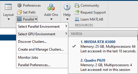
GPUDevice Object: Changes to device properties
gpuDevice objects that the gpuDevice function
returns now have these additional properties:
GraphicsDriverVersion— Graphics driver version currently in use.DriverModel— Operating model of the graphics driver.On Windows operating systems, the model options are:
'WDDM'— Display model.'TCC'— Compute model.
On other operating systems,
DriverModelis'N/A'.CachePolicy— Policy that determines how much GPU memory the GPU can cache to accelerate computation. You can set theCachePolicyproperty to"balanced","minimum", or"maximum".
For example, select a GPU using the gpuDevice function to inspect the new properties.
D = gpuDevice
D =

  CUDADevice with properties:

                      Name: 'NVIDIA RTX A5000'
                     Index: 1
         ComputeCapability: '8.6'
            SupportsDouble: 1
     GraphicsDriverVersion: '511.79'
               DriverModel: 'TCC'
            ToolkitVersion: 11.2000
        MaxThreadsPerBlock: 1024
          MaxShmemPerBlock: 49152 (49.15 KB)
        MaxThreadBlockSize: [1024 1024 64]
               MaxGridSize: [2.1475e+09 65535 65535]
                 SIMDWidth: 32
               TotalMemory: 25553076224 (25.55 GB)
           AvailableMemory: 25145376768 (25.15 GB)
               CachePolicy: 'balanced'
       MultiprocessorCount: 64
              ClockRateKHz: 1695000
               ComputeMode: 'Default'
      GPUOverlapsTransfers: 1
    KernelExecutionTimeout: 0
          CanMapHostMemory: 1
           DeviceSupported: 1
           DeviceAvailable: 1
            DeviceSelected: 1
Change the caching policy to allow the GPU to cache the maximum amount of memory for accelerating computation.
D.CachePolicy = "maximum";The DriverVersion property no longer displays by default, but
you can still query the property using dot notation. There are no plans to remove
the DriverVersion property.
GPU Functionality: Use functions with new and enhanced
gpuArray support
These MATLAB functions have new and enhanced gpuArray support:
eig— You can now provide two input matrices, compute three outputs (eigenvalues, left eigenvectors, and right eigenvectors), specify the output format of the eigenvalues as a matrix or a vector, and provide input matrices containingNaNorInfvalues.interp1— You can now use the"next"and"previous"interpolation methods.mustBeFloat,mustBeGreaterThan,mustBeGreaterThanOrEqual,mustBeInRange,mustBeLessThan,mustBeLessThanOrEqual,mustBeNegative,mustBeNonempty,mustBeNonmissing,mustBeNonnegative,mustBeNonpositive,mustBeNonsparse,mustBeNumeric,mustBeNumericOrLogical,mustBePositive,mustBeReal,mustBeScalarOrEmpty,mustBeVector
For more information, see Run MATLAB Functions on a GPU.
These Statistics and Machine Learning Toolbox functions have new and enhanced gpuArray support:
regress(Statistics and Machine Learning Toolbox)fitrsvm(Statistics and Machine Learning Toolbox) — You can now specifygpuArrayinputs.Most object functions of
RegressionSVM(Statistics and Machine Learning Toolbox),CompactRegressionSVM(Statistics and Machine Learning Toolbox), andRegressionPartitionedSVM(Statistics and Machine Learning Toolbox) run on a GPU when you provide GPU array input arguments. These object functions do not support GPU array input arguments.Object Function Model Type incrementalLearner(Statistics and Machine Learning Toolbox)RegressionSVM(Statistics and Machine Learning Toolbox) andCompactRegressionSVM(Statistics and Machine Learning Toolbox)lime(Statistics and Machine Learning Toolbox)RegressionSVM(Statistics and Machine Learning Toolbox) andCompactRegressionSVM(Statistics and Machine Learning Toolbox)shapley(Statistics and Machine Learning Toolbox)RegressionSVM(Statistics and Machine Learning Toolbox) andCompactRegressionSVM(Statistics and Machine Learning Toolbox)update(Statistics and Machine Learning Toolbox)CompactRegressionSVM(Statistics and Machine Learning Toolbox)You can now use the
gather(Statistics and Machine Learning Toolbox) function to create aRegressionSVM(Statistics and Machine Learning Toolbox),CompactRegressionSVM(Statistics and Machine Learning Toolbox), orRegressionPartitionedSVM(Statistics and Machine Learning Toolbox) object from an equivalent object fitted with GPU array data. The properties of the new object are stored in host memory.
For a list of all Statistics and Machine Learning Toolbox functions with GPU functionality, see Functions with gpuArray
support (Statistics and Machine Learning Toolbox).
These Signal Processing Toolbox functions have new and enhanced gpuArray support:
bandpower(Signal Processing Toolbox)medfreq(Signal Processing Toolbox)obw(Signal Processing Toolbox)powerbw(Signal Processing Toolbox)rssq(Signal Processing Toolbox)signalFrequencyFeatureExtractor(Signal Processing Toolbox)signalTimeFeatureExtractor(Signal Processing Toolbox)sinad(Signal Processing Toolbox)snr(Signal Processing Toolbox)thd(Signal Processing Toolbox)
For a list of all Signal Processing Toolbox functions with GPU functionality, see Functions with gpuArray
support (Signal Processing Toolbox).
These Wavelet Toolbox functions have new and enhanced gpuArray
support:
For a list of all Wavelet Toolbox functions with GPU functionality, see Functions with gpuArray
support (Wavelet Toolbox).
These Communications Toolbox functions have new gpuArray support:
For a list of all Communications Toolbox functions with GPU functionality, see Functions with gpuArray
support (Communications Toolbox).
PTX Build Option for mexcuda: Compile PTX files using
mexcuda
You can now compile parallel thread execution (PTX) files using the mexcuda function by specifying the -ptx build
option. The function compiles the PTX file and gives it the same name as the input
CUDA C++ (CU) source file.
You no longer need to install the CUDA Toolkit to compile a PTX file from a CU file.
For an updated overview of the workflow for creating and executing your own custom
CUDAKernel object, see Run CUDA or PTX Code on GPU.
Support for New GPU Architectures: Update to NVIDIA
CUDA
11.8
Parallel Computing Toolbox software now uses CUDA version 11.8, which supports NVIDIA GPUs with compute capability up to 9.x, including
Hopper architecture GPUs. For more information, see GPU Computing Requirements.
Workflow Examples: New and updated examples and topics
These new and updated examples show how to accelerate your code using a GPU:
Accelerate Linear Model Fitting on GPU (Statistics and Machine Learning Toolbox)
Improve Performance of Small Matrix Problems on the GPU Using
pagefun
This updated example shows how to monitor the training of deep neural networks in
a batch job using a ValueStore object:
Send Deep Learning Batch Job to Cluster (Deep Learning Toolbox)
This new topic helps you choose the right parallel language and workflow for your needs:
Thread-Based Environment: Use new functionality on thread workers
These MATLAB functions and classes now have thread-based support:
For more information, see Run MATLAB Functions in Thread-Based Environment.
Tall Arrays: Use functions with new and enhanced tall array support
Distributed and Tall tables and timetables:
Perform calculations directly on distributed and tall tables and timetables without
extracting their data
You can now perform calculations directly on distributed and tall tables and timetables without extracting their data. In previous releases, all calculations require you to extract data from your distributed and tall tables and timetables by indexing into them.
For example, to scale a distributed table that contains numeric data, multiply it by a scale factor.
table = array2table(rand(2),VariableNames={"V1","V2"});
distTable = distributed(table)
distTable =
2×2 distributed table
V1 V2
_______ ________
0.69483 0.95022
0.3171 0.034446distTable = distTable .* 10
distTable =
  2×2 distributed table
      V1          V2
    _______    ________

    6.9483     9.5022
     3.171    0.34446
These MATLAB functions have new support for performing calculations directly on distributed and tall tables and timetables.
Arithmetic functions –
ceil,fix,floor,ldivide,minus,mod,plus,power,prod,rdivide,rem,round,sum,timesTrigonometric functions –
acos,acosd,acosh,acot,acotd,acoth,acsc,acscd,acsch,asec,asecd,asech,asin,asind,asinh,atan2,atan2d,atand,atanh,cos,cosd,cosh,cospi,cot,cotd,cscd,csch,sec,secd,sech,sin,sind,sinh,sinpi,tan,tand,tanhExponential and logarithmic functions –
exp,expm1,log,log10,log1p,log2,nextpow2,nthroot,pow2,reallog,realpow,realsqrt,sqrtComplex number functions –
abs
For more information about performing calculations directly on tables and timetables, see Direct Calculations on Tables and Timetables.
Composite arrays: Use gather to convert a Composite array into
a local cell array.
You can now use the gather function to convert a Composite array containing data on parallel workers into a cell array
in the local workspace.
For example, gather data after the execution of an spmd
statement.
parpool("Threads",3)
spmd, c = ones(spmdIndex); end
data = gather(c)
data =

  1×3 cell array

{[1]} {2×2 double} {3×3 double}In previous releases, when you use gather on a
Composite array, MATLAB returns the same Composite array as the output.
If you have code that relies on this behavior, update your code to avoid
compatibility issues.
Distributed Arrays: Use functions with new and enhanced distributed array support
These functions have new and enhanced distributed array support:
movmad,movmax,movmean,movmedian,movmin,movprod,movstd,movsum,movvar— You can now use theSamplePointsname-value argument.mpower— You can now use a square matrix for the base or exponent.mustBeFinite,mustBeFloat,mustBeGreaterThan,mustBeGreaterThanOrEqual,mustBeInRange,mustBeInteger,mustBeLessThan,mustBeLessThanOrEqual,mustBeNegative,mustBeNonempty,mustBeNonmissing,mustBeNonNan,mustBeNonnegative,mustBeNonpositive,mustBeNonsparse,mustBeNonzero,mustBeNumeric,mustBeNumericOrLogical,mustBePositive,mustBeReal,mustBeScalarOrEmpty,mustBeVector
For more information, see Run MATLAB Functions with Distributed Arrays.
Discover Clusters Supports Third-Party Schedulers
The Discover Clusters dialog can now locate third-party scheduler clusters for different releases of parallel computing products. For information about cluster discovery, see Discover Clusters.
Third-Party Cluster Schedulers: Access simplified plugin scripts for integration on GitHub
When you integrate MATLAB with your scheduler using MATLAB
Parallel Server, you can now use a single set of scripts and specify the values of one
of these AdditionalProperties properties to describe your
network configuration.
| Network Configuration | Previous Submission Mode | New Properties to Set |
|---|---|---|
The MATLAB client does not share the file system with the cluster nodes. | Shared |
|
The MATLAB client is unable to directly submit jobs to the third-party scheduler. | Remote |
|
The MATLAB client does not share the file system with the cluster nodes and is unable to directly submit jobs to the third-party scheduler. | Nonshared |
|
In previous releases, you have to choose a set of scripts for shared, nonshared, and remote submission modes
The simplified plugin scripts for these third-party schedulers are now available in these GitHub repositories:
You can still download the plugin scripts from MATLAB Central™ File Exchange.
Third-Party Cluster Schedulers: Open ports on workers to listen for connections from client
You can now open listening ports on MATLAB
Parallel Server workers running on third-party scheduler clusters to enable your
MATLAB client to connect to the workers. Use this functionality to run
interactive parallel pools on third-party scheduler clusters without the need to
modify your network systems such as firewalls. For more details, see pctconfig.
LDAP Support for MATLAB Job Scheduler Clusters: Authenticate cluster logins against LDAP credentials
Validate and control user access to a MATLAB Job Scheduler cluster by using a Lightweight Directory Access Protocol (LDAP) server to authenticate user logins. For more information, see Configure LDAP Server Authentication for MATLAB Job Scheduler (MATLAB Parallel Server).
Cluster Security: Restrict use of MATLAB Job Scheduler cluster commands
You can now restrict the use of cluster changing commands to specific users by verifying commands sent to MATLAB Job Scheduler clusters. In previous releases, any user can execute commands that can change the state of cluster. For more information, see Set Cluster Command Verification (MATLAB Parallel Server).
Parallel Computing in MATLAB Online Server Environment: Speed up MATLAB Online workflows
You can now integrate Parallel Computing Toolbox software and MATLAB Parallel Server with your MATLAB Online Server™ instance and use parallel computing to speed up MATLAB Online™ workflows.
MATLAB Parallel Server in Kubernetes: Configure and run MATLAB Parallel Server workers on Kubernetes clusters
You can now integrate MATLAB Parallel Server with your Kubernetes® cluster and interface Parallel Computing Toolbox software on your computer to the Kubernetes cluster. For more details, see the Parallel Computing Toolbox for MATLAB Parallel Server with Kubernetes plugin script on GitHub or MATLAB Central File Exchange.
Functionality being removed or changed
Preferred number of workers in a parallel pool option has been removed
Behavior change
The Preferred number of workers in a parallel pool option in Parallel Preferences has been removed. This change gives you more control over how many workers to start on nonlocal clusters.
For MATLAB Job Scheduler, third party schedulers, and cloud clusters, you can
use the PreferredPoolNumWorkers property of your cluster
profiles to specify the preferred number of workers to start in a parallel pool.
For the local Processes and Threads
profiles, use the NumWorkers property to specify the
default number of workers to start in a parallel pool.
rng("default") on MATLAB parallel workers now sets random number generator settings to
worker default
Behavior change
When you call the rng function with the "default" argument on
MATLAB parallel workers, MATLAB resets the random number generator settings to the worker default
values. The default corresponds to the Threefry generator with 20 rounds and a
seed of 0
In previous releases, when you run rng("default") on
parallel workers, MATLAB changes the worker random number generator settings to the client
default values. The default corresponds to the Mersenne Twister generator with a
seed of 0.
parallel.pool.Constant objects no longer automatically
transferred to workers
Behavior change
MATLAB no longer automatically transfers the parallel.pool.Constant object from your current MATLAB session to workers in a parallel pool. MATLAB sends the Constant object to workers only if the
object is required to execute your code.
Thread-Based Parallel Pool: startup or
matlabrc no longer runs when workers start
Behavior change
When you start a thread-based parallel pool, the thread-based workers no
longer run the startup or matlabrc file.
All startup options on the client are automatically mirrored to the thread-based
workers.
Thread-Based Parallel Pool: Specify number of thread workers using
parpool
You can now specify the pool size of a thread-based parallel pool by using
parpool.
For example, start a pool of four thread workers.
parpool("Threads",4);You can also set Threads as the default parallel environment
and start a parallel pool with the largest possible number of
workers.
parallel.defaultProfile("Threads");
parpool([1 50]);
Parallel menu: Select Threads using the
Parallel menu
You can now select the Threads parallel environment option
from the MATLAB desktop Parallel menu.
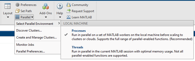
You can set the default parallel environment on your local machine from the MATLAB desktop Home tab, in the Environment area, by selecting one of these options:
Parallel > Select Parallel Environment > Processes
Parallel > Select Parallel Environment > Threads
You can also change the default profile in Parallel Preferences. For more information, see Specify Your Parallel Preferences.
The local profile is no longer recommended. For more
information, see Functionality being removed or changed.
gpuDevice Object: Display values for byte-based memory
properties with appropriate units
The gpuDevice object now displays the TotalMemory,
AvailableMemory, and MaxShmemPerBlock
properties with appropriately scaled units. The object displays these properties as
bytes (B), kilobytes (KB), megabytes (MB), or gigabytes (GB). Accessing any of these
properties using dot notation still returns a value in bytes.
For example, create a gpuDevice object and access its TotalMemory
property.
g = gpuDevice
g =

  CUDADevice with properties:

                      Name: 'NVIDIA RTX A5000'
                     Index: 1
         ComputeCapability: '8.6'
            SupportsDouble: 1
             DriverVersion: 11.6000
            ToolkitVersion: 11.2000
        MaxThreadsPerBlock: 1024
          MaxShmemPerBlock: 49152 (49.15 KB)
        MaxThreadBlockSize: [1024 1024 64]
               MaxGridSize: [2.1475e+09 65535 65535]
                 SIMDWidth: 32
               TotalMemory: 25553076224 (25.55 GB)
           AvailableMemory: 25153765376 (25.15 GB)
       MultiprocessorCount: 64
              ClockRateKHz: 1695000
               ComputeMode: 'Default'
      GPUOverlapsTransfers: 1
    KernelExecutionTimeout: 0
          CanMapHostMemory: 1
           DeviceSupported: 1
           DeviceAvailable: 1
            DeviceSelected: 1
g.TotalMemory
ans =

   2.5553e+10
GPU Workflow Examples: New and updated examples and topics
These new and updated examples and topics show how to accelerate your code using a GPU:
Cloud GPU Computing: Access Cloud GPUs and Clusters in AWS Using Cloud Center
If you do not have a GPU available, you can speed up your MATLAB code with one or more high-performance NVIDIA GPUs in the cloud. Working in the cloud requires some initial setup, but using cloud resources can significantly accelerate your code without requiring you to buy and set up your own local GPUs. The simplest way to access a high-performance cloud GPU is to use Cloud Center.
From April 2022, you can use Cloud Center to start MATLAB in Amazon Web Services (AWS). You can start a single machine, with MATLAB installed, that you can access from a web browser or a remote desktop application. To get started, see Get Started with Cloud Center and Start MATLAB on Amazon Web Services (AWS) Using Cloud Center. To learn more about other cloud options for GPU access, see Run MATLAB using GPUs in the Cloud.
You can continue to use Cloud Center to start and manage MATLAB Parallel Server clusters that you can access from any MATLAB client. MATLAB Parallel Server clusters provide more hardware, including GPU and CPU clusters.
New Examples: Use ValueStore to monitor
batch jobs
These new examples show how to retrieve data and monitor
batch jobs with a ValueStore object:
Monitor Batch Jobs with
ValueStoreshows how to useValueStoreto update a waitbar.Monitor Monte Carlo Batch Jobs with ValueStore shows how to use
ValueStoreto access and monitor data from a batch Monte Carlo simulation.
Parallel workflow examples: Use clusters for 5G Communications simulations
This new Communications Toolbox example shows how to accelerate simulations using clusters for 5G LDPC Block Error Rate:
5G LDPC Block Error Rate Simulation Using the Cloud or a Cluster (Communications Toolbox)
Data Analysis: Use mapreduce on Spark clusters
Parallel Computing Toolbox and MATLAB
Parallel Server support the use of Spark clusters for the execution environment of
mapreduce applications. For more information, see:
Configure a Spark Cluster (MATLAB Parallel Server)
Parallel Computing page: Learn about MathWorks solutions that help you take advantage of more hardware resources
Use the new Parallel Computing page to discover solutions that use parallel, GPU, and cloud computing.
Multistep Authentication for Third-Party Schedulers: Connect to remote clients with multiple authentication options
You can now use a RemoteClusterAccess object to perform multistep authentication with
any number of authentication options. To connect to a cluster with multiple
authentication requirements, specify the AuthenticationMode
property of the RemoteClusterAccess object as a string array or
cell array containing a combination of "Agent",
"IdentityFile", "Multifactor", and
"Password".
For example, create a RemoteClusterAccess object to connect to a
cluster that requires a password and identity
file.
RemoteClusterAccess(AuthenticationMode={"IdentityFile","Password"}); The sample plugin scripts for third-party schedulers now accept the cell array
{"IdentityFile","Password"} as the value of the
AuthenticationMode property of an
AdditionalProperties object, which sets the same
AuthenticationMode property value in the
RemoteClusterAccess object.
Thread-Based Environment: Use new functionality on thread workers
These Parallel Computing Toolbox functions now have new thread-based support:
These Image Processing Toolbox functions now have thread-based support.
adapthisteq (Image Processing Toolbox) | bfscore (Image Processing Toolbox) | bwconncomp (Image Processing Toolbox) | bwdist (Image Processing Toolbox) |
bwferet (Image Processing Toolbox) | bwlabel (Image Processing Toolbox) | bwlabeln (Image Processing Toolbox) | bwlookup (Image Processing Toolbox) |
bwmorph3 (Image Processing Toolbox) | bwpack (Image Processing Toolbox) | bwskel (Image Processing Toolbox) | bwtraceboundary (Image Processing
Toolbox) |
bwunpack (Image Processing Toolbox) | demosaic (Image Processing Toolbox) | edge (Image Processing Toolbox) | edge3 (Image Processing Toolbox) |
entropyfilt (Image Processing Toolbox) | exrHalfAsSingle (Image Processing
Toolbox) | exrinfo (Image Processing Toolbox) | exrread (Image Processing Toolbox) |
exrwrite (Image Processing Toolbox) | fibermetric (Image Processing Toolbox) | grabcut (Image Processing Toolbox) | histeq (Image Processing Toolbox) |
hough (Image Processing Toolbox) | imabsdiff (Image Processing Toolbox) | imapplymatrix (Image Processing Toolbox) | imbothat (Image Processing Toolbox) |
imboxfilt (Image Processing Toolbox) | imboxfilt3 (Image Processing Toolbox) | imclose (Image Processing Toolbox) | imdiffusefilt (Image Processing Toolbox) |
imdilate (Image Processing Toolbox) | imerode (Image Processing Toolbox) | imfill (Image Processing Toolbox) | imfilter (Image Processing Toolbox) |
imgaussfilt (Image Processing Toolbox) | imgaussfilt3 (Image Processing Toolbox) | imgradient (Image Processing Toolbox) | imgradient3 (Image Processing Toolbox) |
imhist (Image Processing Toolbox) | imlincomb (Image Processing Toolbox) | imnlmfilt (Image Processing Toolbox) | imopen (Image Processing Toolbox) |
imreconstruct (Image Processing Toolbox) | imregionalmax (Image Processing Toolbox) | imregionalmin (Image Processing Toolbox) | imsegfmm (Image Processing Toolbox) |
imtophat (Image Processing Toolbox) | inpaintCoherent (Image Processing
Toolbox) | inpaintExemplar (Image Processing
Toolbox) | integralImage (Image Processing Toolbox) |
integralImage3 (Image Processing
Toolbox) | intlut (Image Processing Toolbox) | iradon (Image Processing Toolbox) | isexr (Image Processing Toolbox) |
label2idx (Image Processing Toolbox) | medfilt2 (Image Processing Toolbox) | medfilt3 (Image Processing Toolbox) | modefilt (Image Processing Toolbox) |
multissim (Image Processing Toolbox) | multissim3 (Image Processing Toolbox) | nitfread (Image Processing Toolbox) | obliqueslice (Image Processing Toolbox) |
ordfilt2 (Image Processing Toolbox) | planar2raw (Image Processing Toolbox) | poly2mask (Image Processing Toolbox) | qtdecomp (Image Processing Toolbox) |
radon (Image Processing Toolbox) | raw2planar (Image Processing Toolbox) | raw2rgb (Image Processing Toolbox) | rawread (Image Processing Toolbox) |
regionprops (Image Processing Toolbox) | regionprops3 (Image Processing Toolbox) | rgb2lab (Image Processing Toolbox) | rgb2lightness (Image Processing Toolbox) |
superpixels (Image Processing Toolbox) | superpixels3 (Image Processing Toolbox) | watershed (Image Processing Toolbox) |
For more information, see Run MATLAB Functions in Thread-Based Environment.
GPU Functionality: Use functions with new and enhanced
gpuArray support
These MATLAB functions have new and enhanced gpuArray support:
rmoutliers- Support for defining outlier locations and returning the outlier indicator, thresholds, and center value outputs
For more information, see Run MATLAB Functions on a GPU.
These Statistics and Machine Learning Toolbox functions have enhanced gpuArray support:
fitcecoc(Statistics and Machine Learning Toolbox) - Support for categorical predictors for classification tree learnersfitcensemble(Statistics and Machine Learning Toolbox) - Support for categorical predictors for classification tree learnersfitcsvm(Statistics and Machine Learning Toolbox)Support for hyperparameter optimization
When
fitcsvmfits the SVM model on a GPU, some of the properties of theClassificationSVM(Statistics and Machine Learning Toolbox) model are stored in GPU memoryUse
gatherto create aClassificationSVMorCompactClassificationSVMobject with properties stored in the local workspace from an equivalent object with properties stored in GPU memory
fitctree(Statistics and Machine Learning Toolbox) - Support for categorical predictorsfitensemble(Statistics and Machine Learning Toolbox) - Support for categorical predictorsfitrensemble(Statistics and Machine Learning Toolbox) - Support for categorical predictorsfitrtree(Statistics and Machine Learning Toolbox) - Support for categorical predictorspca(Statistics and Machine Learning Toolbox) - Improved performance when you use the SVD algorithmObject functions of the
CompactClassificationSVM(Statistics and Machine Learning Toolbox) model execute on a GPU if the model is fitted with GPU arraysObject functions of the
ClassificationSVM(Statistics and Machine Learning Toolbox) model execute on a GPU if the model is fitted with GPU arrays
For a list of all Statistics and Machine Learning Toolbox functions with GPU functionality, see Functions with gpuArray
support (Statistics and Machine Learning Toolbox).
These Signal Processing Toolbox functions have new and enhanced gpuArray support:
For a list of all Signal Processing Toolbox functions with GPU functionality, see Functions with gpuArray
support (Signal Processing Toolbox).
This Audio Toolbox function has enhanced gpuArray support :
audioFeatureExtractor(Audio Toolbox) - Code acceleration support forzerocrossrate
For a list of all Audio Toolbox functions with GPU functionality, see Functions with gpuArray
support (Audio Toolbox).
This Image Processing Toolbox function has new gpuArray support:
gray2ind(Image Processing Toolbox)
For a list of all Image Processing Toolbox functions with GPU functionality, see Functions with gpuArray
support (Image Processing Toolbox).
Tall Arrays: Use functions with new and enhanced tall array support
These functions have new and enhanced tall array support:
rmoutliers- Support for defining outlier locations and returning the outlier indicator, thresholds, and center value outputsround- Support for specifying a direction for rounding ties
For more information, see Tall Arrays.
Distributed Arrays: Use functions with new and enhanced distributed array support
These functions have new and enhanced distributed array support:
round- Support for specifying a direction for breaking ties
For more information, see Run MATLAB Functions with Distributed Arrays.
MATLAB Job Scheduler: Support for your own Java installation
You can now use your own Java 8 installation with MATLAB Job Scheduler (MJS). To use your own Java 8 installation with MJS, specify a path to a Java Runtime Environment (JRE) installation for the
MJS_Java variable in your mjs_def file.
For more information on where to find the mjs_def file, see Customize Startup Parameters (MATLAB Parallel Server).
Element-Wise Operations: Improved performance on GPU
Element-wise operations on large numbers of gpuArray objects
show improved performance. Improvements are greater when you operate on large
numbers of gpuArray objects. For example, adding one to every
element of a cell array of the gpuArray data in this function is
about 43.8x faster than in the previous release:
function timeElementWiseOps

% Prepare a cell array of gpuArray data
x = cell(5000,1);
x = cellfun(@(z) rand(10,"gpuArray"),x,"UniformOutput",false);

% Make all arrays different to one another
x = cellfun(@(z) z+rand(1,"gpuArray"),x,"UniformOutput",false);

% Time adding one to each element
gputimeit(@() cellfun(@(z) z+1,x,"UniformOutput",false))

end
The approximate execution times are:
R2022a: 5.70 seconds
R2022b: 0.13 seconds
The code was timed on a Windows 10, Intel
Xeon W-2133 @ 3.60 GHz test system with an NVIDIA RTX A5000 GPU by calling the timeElementWiseOps
function.
svd Function: Improved performance on GPU
The svd function shows improved performance when called with a
gpuArray input matrix that is short and wide (n >
3m) or tall and narrow (m > 6n). For example,
performing a singular value decomposition of a matrix in this function is about 1.4x
faster than in the previous release:
function timeSVD

% Prepare input matrix
A = rand(1000,10000,"gpuArray");

% Time SVD
gputimeit(@() svd(A),3)

end
The approximate execution times are:
R2022a: 2.64 seconds
R2022b: 1.88 seconds
The code was timed on a Windows 10, Intel
Xeon W-2133 @ 3.60 GHz test system with an NVIDIA RTX A5000 GPU by calling thetimeSVD
function.
Functionality being removed or changed
labXxx functions are not recommended and are renamed to
spmdXxx
Still runs
To align these function names with their intended use within
spmd blocks, these spmd block code
execution and communication functions have been renamed:
These functions are no longer recommended, but they will continue to work. This table shows the recommended replacement functions.
| Functionality | Recommended Replacement | Compatibility Considerations |
|---|---|---|
labBarrier | spmdBarrier | Replace all instances of labBarrier with
spmdBarrier |
labBroadcast | spmdBroadcast | Replace all instances of labBroadcast
with spmdBroadcast |
labindex | spmdIndex | Replace all instances of labindex with
spmdIndex |
labProbe | spmdProbe | Replace all instances of labProbe with
spmdProbe |
labReceive | spmdReceive | Replace all instances of labReceive with
spmdReceive |
labSend | spmdSend | Replace all instances of labSend with
spmdSend |
labSendReceive | spmdSendReceive | Replace all instances of labSendReceive
with spmdSendReceive |
numlabs | spmdSize | Replace all instances of numlabs with
spmdSize |
The labXxx functions will not be removed.
gcat, gop, and
gplus are not recommended and are renamed to
spmdCat, spmdReduce, and
spmdPlus
Still runs
local profile has been renamed to
Processes on the Parallel menu
Still runs
For a process-based parallel environment on a local machine, the
local profile is no longer recommended. Use
Processes instead.
To start a parallel pool of process workers, use this code.
In previous releases, you used this code which is no longer recommended.parpool("Processes")parpool("local")
The local profile option has been removed from
the Parallel menu but will continue to work when you
use it programmatically.
parallel.defaultClusterProfile and
parallel.clusterProfiles are renamed to
parallel.defaultProfile and
parallel.listProfiles
Still runs
The parallel.defaultClusterProfile and parallel.clusterProfiles functions are renamed.
parallel.defaultClusterProfile is renamed to parallel.defaultProfile.
parallel.clusterProfiles is renamed to parallel.listProfiles. The
parallel.defaultClusterProfile and
parallel.clusterProfiles will not be removed.
To update your code, replace all instances of
parallel.defaultClusterProfile with
parallel.defaultProfile and
parallel.clusterProfiles with
parallel.listProfiles.
remotecopy has been removed
Errors
Starting in R2022b, remotecopy (MATLAB Parallel Server) has been removed. To copy
files to and from a remote host, use scp or
sftp instead.
Previously you used
remotecopyand-protocol scpto copy files to and from a remote host using the secure copy protocol (SCP).This table shows how to use
scpinstead.Errors Recommended remotecopy -remotehost host1 -local /my/file/path -to -remote /remote/file/path -protocol scp
scp /my/file/path host1:/remote/file/path
remotecopy -remotehost host1,host2 -local /my/file/path -to -remote /remote/file/path -protocol scp
scp /my/file/path host1:/remote/file/path
scp /my/file/path host2:/remote/file/path
remotecopy -remotehost host1 -local /my/file/path -from -remote /remote/file/path -protocol scp
scp host1:/remote/file/path /my/file/path
Previously you used
remotecopyand-protocol sftpto copy files to and from a remote host using the secure file transfer protocol (SFTP).This table shows how to use
sftpinstead.Errors Recommended remotecopy -remotehost host1 -local /my/file/path -to -remote /remote/file/path -protocol sftp
sftp /my/file/path host1:/remote/file/path
remotecopy -remotehost host1,host2 -local /my/file/path -to -remote /remote/file/path -protocol sftp
sftp /my/file/path host1:/remote/file/path
sftp /my/file/path host2:/remote/file/path
remotecopy -remotehost host1 -local /my/file/path -from -remote /remote/file/path -protocol sftp
sftp host1:/remote/file/path /my/file/path
remotemjs has been removed
Errors
Starting in R2022b, remotemjs (MATLAB Parallel Server) has been removed. Use
ssh instead.
Previously you used remotemjs to run MATLAB Job Scheduler commands on a remote host using -protocol
ssh or -protocol winsc.
This table shows how to use ssh instead.
| Errors | Recommended |
|---|---|
remotemjs <mjs options> -matlabroot <installfoldername> -remotehost host1 |
ssh host1 <installfoldername>/toolbox/parallel/bin/mjs <mjs options> |
remotemjs <mjs options> -matlabroot <installfoldername> -remotehost host1,host2 |
ssh host1 <installfoldername>/toolbox/parallel/bin/mjs <mjs options> ssh host2 <installfoldername>/toolbox/parallel/bin/mjs <mjs options> |
ValueStore and FileStore objects: Retrieve
data and files on MATLAB clients during job execution
ValueStore and FileStore objects now allow you to store data and files from
MATLAB workers that can be retrieved by MATLAB clients during the execution of a job (even while the job is still
running). These objects are not held in system memory, so they can be used to store
large results. A FileStore object provides a universal location
for workers to copy files. MATLAB clients can then access these files regardless of
the specific cluster environment where the worker is running.
The ValueStore and FileStore objects are
automatically created when you create a job on a cluster, a parallel pool of process
workers on your local machine, or a parallel pool of workers on a cluster of
machines. To access the ValueStore and
FileStore objects on a worker, use the getCurrentValueStore and getCurrentFileStore functions, respectively.
Multifactor Authentication for the Generic Scheduler Interface: Connect to remote
clients with RemoteClusterAccess using two or more authentication
factors
RemoteClusterAccess objects now allow you to perform multifactor
authentication, including two-factor authentication. To do so, specify
'Multifactor' for the AuthenticationMode
name-value argument. For details, see the RemoteClusterAccess
reference page. The sample plugin scripts for third-party schedulers now accept
'Multifactor' as the value for the
AuthenticationMode property of
AdditionalProperties, which sets that value on
RemoteClusterAccess.
Cluster resizing: Customize your MATLAB Job Scheduler cluster to resize automatically
You can customize your MATLAB Job Scheduler (MJS) cluster to resize automatically. After you set up auto-resizing, also called auto-scaling, the cluster can automatically change the number of workers with the amount of work submitted. The cluster grows (scales up) when there is more work to do and shrinks (scales down) when there is less work to do. This allows you to use your compute resources more efficiently and can result in cost savings. To learn more, see Set up MATLAB Job Scheduler Cluster for Auto-Resizing (MATLAB Parallel Server).
Parallel Pools: Check status of pools
Starting in R2022a, you can query if any type of pool is currently running by
using the Busy property of the pool. This property indicates
whether the parallel pool is busy, specified as true or
false. The pool is busy if there is outstanding work for the
pool to complete.
Background Pool: Number of thread workers no longer limited to 8 workers
Before R2022a, the NumWorkers property was capped at a maximum
of 8 workers when Parallel Computing Toolbox was installed, and 1 worker when not installed. This limit is no
longer in place when the Parallel Computing Toolbox is installed. When Parallel Computing Toolbox is not installed, the background pool remains limited to 1
worker.
Thread-Based Parallel Pool: See futures in active pool
Starting in R2022a, you can query all queued and running futures on a parallel
pool by using the FevalQueue property of the pool. To create
futures, use parfeval and parfevalOnAll. For more information on futures, see Future.
cancelAll Method: Cancel currently queued and running futures
in a parallel pool
cancelAll cancels all futures currently queued or running in a
parallel pool. Queued or running futures are listed in the
FevalQueue property.
For example, you can use cancelAll to stop all
Futures in an FevalQueue.
pool = parpool;
cancelAll(pool.FevalQueue);
GPU Functionality: Use new and enhanced gpuArray
functions
New GPU support in MATLAB:
For more information, see Run MATLAB Functions on a GPU.
New GPU support in Statistics and Machine Learning Toolbox:
fitensemble(Statistics and Machine Learning Toolbox)fitrensemble(Statistics and Machine Learning Toolbox)New support for probability functions:
gev*,gp*,nbin*
For a list of all Statistics and Machine Learning Toolbox functions with GPU functionality, see Functions with gpuArray
support (Statistics and Machine Learning Toolbox).
The following functions have new and enhanced gpuArray support in
Signal Processing Toolbox:
For a list of all Signal Processing Toolbox functions with GPU functionality, see Functions with gpuArray
support (Signal Processing Toolbox).
The following functions have new gpuArray support in Audio Toolbox:
pitch(Audio Toolbox)audioDataAugmenter(Audio Toolbox)audioFeatureExtractor(Audio Toolbox) - improved support
For a list of all Audio Toolbox functions with GPU functionality, see Functions with gpuArray
support (Audio Toolbox).
The following functions have new gpuArray and
dlArray support in Wavelet Toolbox:
For a list of all Wavelet Toolbox functions with GPU functionality, see Functions with gpuArray
support (Wavelet Toolbox).
Support for NVIDIA
CUDA
11.2: Update to CUDA Toolkit 11.2
The parallel computing products now use CUDA toolkit version 11.2. To generate CUDA kernel objects from CU code or compile CUDA compatible source code, libraries, and executables using GPU Coder™, you must use toolkit version 11.2. For more
information, see Run CUDA or PTX Code on GPU.
Distributed Arrays: Use new and enhanced distributed array functionality
Parallel Features in Other Products
Parallel features added in other products:
Experiment Manager: Offload deep learning experiments as batch jobs in a cluster
Starting in R2022a, Experiment Manager (Deep Learning Toolbox) supports offloading experiments as batch jobs in a cluster. You can configure the cluster to run multiple trials at the same time or to run a single trial at a time on multiple parallel workers. While the experiment is running in the cluster, you can run other experiments, close the app and continue using MATLAB, or close your MATLAB session. For more information, see Offload Experiments as Batch Jobs to Cluster (Deep Learning Toolbox).
Parallel Simulations: Perform parameter sweeps using Parameter Combinations
In R2022a, you can use Parameter Combinations in the Multiple Simulations panel of the Simulink® Editor for workflows with multiple simulations, such as Monte-Carlo simulations and parameter sweeps. Parameter Combinations allows you to create sequential and exhaustive combinations of parameters, specify value ranges, and run simulations with these combinations. The Multiple Simulations panel was introduced in R2021b. For more information, see Multiple Simulations Panel: Simulate for Different Values of Stiffness for a Vehicle Dynamics System (Simulink).
Machine Learning Apps: Train draft models in parallel or train in the background to keep the app responsive
In Classification Learner (Statistics and Machine Learning Toolbox) and Regression Learner (Statistics and Machine Learning Toolbox), you can train multiple draft models in parallel. You can use the Use Parallel or Use Background buttons while training models.
Solving Linear System: Improved performance when solving linear systems
A*X = B with gpuArray for symmetric
positive definite matrices A
Solving a linear system of the form A*X = B with
gpuArray by executing A\B shows improved
performance when A is a symmetric positive definite
matrix.
For example, this code solves A*X = B for a 10,000-by-10,000
symmetric positive definite matrix A and a 10,000-by-1 column
vector B. The code is about 2.4x faster than in the previous
release.
function timingTest
rng default
R = rand(10000,"gpuArray");
A = R'*R;
B = ones(10000,1,"gpuArray");
X = A\B;
end
The approximate execution times are:
R2021b: 1.03 s
R2022a: 0.43 s
The code was timed on a Windows 10, Intel
Xeon CPU E5-1640 v3 @ 3.50 GHz with an NVIDIA Titan V GPU test system using the gputimeit
function:
gputimeit(@timingTest)
Functionality being removed or changed
distcomp folder removed, now named
parallel
The distcomp folder has been removed.
In R2019b, the Parallel Computing Toolbox folder was renamed. Since then, the name of the toolbox folder has
been parallel. If you need to reference the location of the
toolbox, update your references to use toolbox/parallel
instead of toolbox/distcomp.
Parallel Language in MATLAB: Share parallel code with any MATLAB user
From R2021b, you can use more parallel language features in serial without Parallel Computing Toolbox. To scale up and speed up computations that use these features, use parallel pools and Parallel Computing Toolbox.
Additionally, you can now share parallel code with other MATLAB users who do not have Parallel Computing Toolbox.
The following features are now available in MATLAB:
parfevaland related functionality such asafterEachandafterAllparallel.pool.DataQueue,parallel.pool.PollableDataQueue, and related functionality such asafterEach
For more information, see Background Processing and Write Portable Parallel Code.
GPU Functionality: Use new and enhanced gpuArray
functions
GPU Functionality: Use new and enhanced gpuArray functions
in Statistics and Machine Learning Toolbox
betafit(Statistics and Machine Learning Toolbox)fitcecoc(Statistics and Machine Learning Toolbox)fitcensemble(Statistics and Machine Learning Toolbox)fitctree(Statistics and Machine Learning Toolbox)fitdist(Statistics and Machine Learning Toolbox)fitrtree(Statistics and Machine Learning Toolbox)gevfit(Statistics and Machine Learning Toolbox)gpfit(Statistics and Machine Learning Toolbox)ksdensity(Statistics and Machine Learning Toolbox)mle(Statistics and Machine Learning Toolbox)mvksdensity(Statistics and Machine Learning Toolbox)nbinfit(Statistics and Machine Learning Toolbox)
For a list of all Statistics and Machine Learning Toolbox functions with GPU functionality, see Functions with gpuArray
support (Statistics and Machine Learning Toolbox).
GPU Functionality: Use new and enhanced gpuArray functions
for working with signals and audio
The following functions have new and enhanced
gpuArraysupport in Signal Processing Toolbox: For a list of all Signal Processing Toolbox functions with GPU functionality, see Functions withgpuArraysupport (Signal Processing Toolbox).downsample(Signal Processing Toolbox)filtfilt(Signal Processing Toolbox)pspectrum(Signal Processing Toolbox)resample(Signal Processing Toolbox)shiftdata(Signal Processing Toolbox)unshiftdata(Signal Processing Toolbox)upfirdn(Signal Processing Toolbox)upsample(Signal Processing Toolbox)xspectrogram(Signal Processing Toolbox)
The following functions have new
gpuArraysupport in Audio Toolbox:classifySound(Audio Toolbox)crepePostprocess(Audio Toolbox)crepePreprocess(Audio Toolbox)detectSpeech(Audio Toolbox)harmonicRatio(Audio Toolbox)openl3Features(Audio Toolbox)openl3Preprocess(Audio Toolbox)pitchnn(Audio Toolbox)vggishFeatures(Audio Toolbox)vggishPreprocess(Audio Toolbox)yamnetPreprocess(Audio Toolbox)
For a list of all Audio Toolbox functions with GPU functionality, see Functions with
gpuArraysupport (Audio Toolbox).
Memory Usage: Use whos to check memory used by
gpuArray and distributed variables
You can now use the whos function to check the amount of memory used by
gpuArray and distributed variables.
Previously, the Bytes variable of the output of
whos showed the number of bytes of the pointer to the
variable in the local memory of the host machine. Now, the Bytes
variable displays the amount of GPU or distributed memory allocated to that
variable. For gpuArray variables, whos
displays the amount of GPU memory used by that variable. For
distributed variables, whos displays the
total memory used by that variable across all workers in the pool.
Distributed Arrays: Use new and enhanced distributed array functionality
decomposition– Support for new decompositionsFor dense matrices, new support for banded decomposition and permuted triangular decomposition
For sparse matrices, new support for LDL decomposition and QR decomposition
For more information, see Run MATLAB Functions with Distributed Arrays.
Thread-Based Environment: Use new and enhanced functionality on threads for working with audio, video, and images
The following MATLAB functions have new and enhanced thread support:
imread– Support for JPEG 2000 (J2C, J2K, JP2, JPF, JPX) format images on threads
The following functions and objects have new thread support in Image Processing Toolbox:
imcrop(Image Processing Toolbox)imcrop3(Image Processing Toolbox)imresize3(Image Processing Toolbox)imrotate(Image Processing Toolbox)imrotate3(Image Processing Toolbox)imtranslate(Image Processing Toolbox)impyramid(Image Processing Toolbox)imwarp(Image Processing Toolbox)affineOutputView(Image Processing Toolbox)findbounds(Image Processing Toolbox)fliptform(Image Processing Toolbox)makeresampler(Image Processing Toolbox)maketform(Image Processing Toolbox)tformarray(Image Processing Toolbox)tformfwd(Image Processing Toolbox)tforminv(Image Processing Toolbox)imregconfig(Image Processing Toolbox)imregcorr(Image Processing Toolbox)imregdemons(Image Processing Toolbox)imregmtb(Image Processing Toolbox)normxcorr2(Image Processing Toolbox)MattesMutualInformation(Image Processing Toolbox)MeanSquares(Image Processing Toolbox)RegularStepGradientDescent(Image Processing Toolbox)OnePlusOneEvolutionary(Image Processing Toolbox)cpcorr(Image Processing Toolbox)cpstruct2pairs(Image Processing Toolbox)fitgeotrans(Image Processing Toolbox)imref2d(Image Processing Toolbox)imref3d(Image Processing Toolbox)affine2d(Image Processing Toolbox)affine3d(Image Processing Toolbox)projective2d(Image Processing Toolbox)gray2ind(Image Processing Toolbox)ind2gray(Image Processing Toolbox)mat2gray(Image Processing Toolbox)label2rgb(Image Processing Toolbox)imsplit(Image Processing Toolbox)adaptthresh(Image Processing Toolbox)otsuthresh(Image Processing Toolbox)imquantize(Image Processing Toolbox)grayslice(Image Processing Toolbox)im2int16(Image Processing Toolbox)im2single(Image Processing Toolbox)im2uint16(Image Processing Toolbox)im2uint8(Image Processing Toolbox)
For more information, see Run MATLAB Functions in Thread-Based Environment.
Functionality Being Removed or Changed
parfeval and parfevalOnAll can now
run in serial with no pool
Behavior change
Starting in R2021b, you can now run parfeval and parfevalOnAll in serial with no pool. This behavior allows you
to share parallel code that you write with users who do not have Parallel Computing Toolbox.
When you use the syntaxes parfeval(fcn,n,X1,...,Xm) or
parfevalOnAll(fcn,n,X1,...,Xm), MATLAB tries to use an open parallel pool if you have Parallel Computing Toolbox. If a parallel pool is not open, MATLAB will create one if automatic pool creation is enabled.
If parallel pool creation is disabled or if you do not have Parallel Computing Toolbox, the function is evaluated in serial. In previous releases, MATLAB threw an error instead.
mldivide and decomposition now
produce the same results for distributed arrays
Behavior change
Starting in R2021b, mldivide and
decomposition now produce the same results when you run
the following code using distributed arrays A and
b.
X = A \ b;
X = decomposition(A) \ b;
decomposition before
mldivide for a non-square distributed matrix
A.Default behavior for decomposition has changed for
distributed arrays
Behavior change
Starting in R2021b, the algorithm for decomposition with
type set to 'auto' (default) has changed for distributed
array input. You see this behavior change when you use
decomposition to decompose a distributed matrix that is
Hermitian, banded, or permuted triangular.
When you use decomposition(A) or
decomposition(A,'auto') with a distributed matrix
A, the type of decomposition selected by MATLAB is limited to the supported decomposition types for distributed arrays.
For a distributed dense matrix
A, in the syntaxdecomposition(A,type)the decomposition types'ldl','cod', and'hessenberg'are not supported.For a distributed sparse matrix
A, in the syntaxdecomposition(A,type)the decomposition types'chol','cod', and'hessenberg'are not supported.