decsg

Decompose constructive solid 2-D geometry into minimal regions

Syntax

dl = decsg(gd,sf,ns)

dl = decsg(gd)

[dl,bt] = decsg(___)

Description

dl = decsg(gd,sf,ns) decomposes the geometry description matrix gd into the geometry matrix dl and returns the minimal regions that satisfy the set formula sf. The name-space matrix ns is a text matrix that relates the columns in gd to variable names in sf.

Typically, you draw a geometry in the PDE Modeler app, then export it to the MATLAB^® Command Window by selecting Export Geometry Description, Set Formula, Labels from the Draw menu in the app. The resulting geometry description matrix gd represents the CSG model. decsg analyzes the model and constructs a set of disjointed minimal regions bounded by boundary segments and border segments. This set of minimal regions constitutes the decomposed geometry and allows other Partial Differential Equation Toolbox™ functions to work with the geometry.

Alternatively, you can use the decsg function when creating a geometry without using the app. See 2-D Geometry Creation at Command Line for details.

To return all minimal regions (sf corresponds to the union of all shapes in gd), use the shorter syntax dl = decsg(gd).

[dl,bt] = decsg(___) returns a Boolean table (matrix) that relates the original shapes to the minimal regions. A column in bt corresponds to the column with the same index in gd. A row in bt corresponds to the index of a minimal region. You can use bt to remove boundaries between subdomains.

Examples

Decompose Geometry Created in PDE Modeler App

Create a 2-D geometry in the PDE Modeler app, then export it to the MATLAB workspace and decompose it to minimal regions by using decsg.

Start the PDE Modeler app and draw a unit circle and a unit square.

pdecirc(0,0,1)
pderect([0 1 0 1])

Enter C1-SQ1 in the Set formula field.

Export the geometry description matrix, set formula, and name-space matrix to the MATLAB workspace by selecting the Export Geometry Description option from the Draw menu.

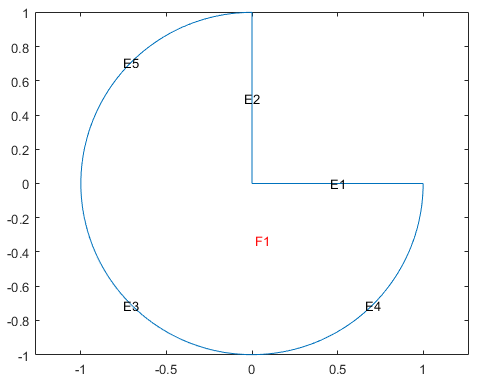
Decompose the exported geometry into minimal regions. The result is one minimal region with five edge segments: three circle edge segments and two line edge segments.

dl = decsg(gd,sf,ns)

dl =
     2.0000   2.0000    1.0000    1.0000    1.0000
          0        0   -1.0000    0.0000    0.0000
     1.0000        0    0.0000    1.0000   -1.0000
          0   1.0000   -0.0000   -1.0000    1.0000
          0        0   -1.0000         0   -0.0000
          0        0    1.0000    1.0000    1.0000
     1.0000   1.0000         0         0         0
          0        0         0         0         0
          0        0         0         0         0
          0        0    1.0000    1.0000    1.0000

View the geometry. Display the edge labels and the face labels.

pdegplot(dl,"EdgeLabels","on","FaceLabels","on")
axis equal

For comparison, decompose the same geometry without specifying the set formula sf and the name-space matrix ns. This syntax returns the union of all shapes in the geometry gd.

dl_all = decsg(gd)

dl_all =
    2.0000    2.0000    2.0000    2.0000    1.0000    1.0000    1.0000    1.0000
         0    1.0000    1.0000         0   -1.0000    0.0000    1.0000    0.0000
    1.0000    1.0000         0         0    0.0000    1.0000    0.0000   -1.0000
         0         0    1.0000    1.0000   -0.0000   -1.0000         0    1.0000
         0    1.0000    1.0000         0   -1.0000         0    1.0000   -0.0000
    3.0000    2.0000    2.0000    3.0000    1.0000    1.0000    3.0000    1.0000
    1.0000         0         0    1.0000         0         0    2.0000         0
         0         0         0         0         0         0         0         0
         0         0         0         0         0         0         0         0
         0         0         0         0    1.0000    1.0000    1.0000    1.0000

View the resulting geometry.

pdegplot(dl_all,"EdgeLabels","on","FaceLabels","on")
axis equal

Remove Boundaries Between Subdomains

Start the PDE Modeler app and draw a unit circle and a unit square.

pdecirc(0,0,1) 
pderect([0 1 0 1])

Enter C1+SQ1 in the Set formula field.

Export the Geometry Description matrix, set formula, and Name Space matrix to the MATLAB workspace by selecting the Export Geometry Description option from the Draw menu.

Decompose the exported geometry into minimal regions. Because the geometry is a union of all regions, C1+SQ1, you can omit the arguments specifying the set formula and name-space matrix when using decsg.

[dl,bt] = decsg(gd)

dl =
    2.0000    2.0000    2.0000    2.0000    1.0000    1.0000    1.0000    1.0000
         0    1.0000    1.0000         0   -1.0000    0.0000    1.0000    0.0000
    1.0000    1.0000         0         0    0.0000    1.0000    0.0000   -1.0000
         0         0    1.0000    1.0000   -0.0000   -1.0000         0    1.0000
         0    1.0000    1.0000         0   -1.0000         0    1.0000   -0.0000
    3.0000    2.0000    2.0000    3.0000    1.0000    1.0000    3.0000    1.0000
    1.0000         0         0    1.0000         0         0    2.0000         0
         0         0         0         0         0         0         0         0
         0         0         0         0         0         0         0         0
         0         0         0         0    1.0000    1.0000    1.0000    1.0000

bt =
     1     0
     0     1
     1     1

View the geometry. Display the edge labels and the face labels.

pdegplot(dl,"EdgeLabels","on","FaceLabels","on")
axis equal

Remove the subdomain boundaries by using the csgdel function.

[dl2,bt2] = csgdel(dl,bt);

View the resulting geometry.

figure
pdegplot(dl2,"EdgeLabels","on","FaceLabels","on")
axis equal

Input Arguments

gd — Geometry description matrix

matrix of double-precision numbers

Geometry description matrix, specified as a matrix of double-precision numbers. The number of columns corresponds to the number of shapes used to construct the geometry. Each column in the geometry description matrix corresponds to a shape in the CSG model. The model supports four types of shapes:

• For a circle, the first row contains 1. The second and third rows contain the x- and y-coordinates of the center. The fourth row contains the radius of the circle.

• For a polygon, the first row contains 2. The second row contains n, which is the number of line segments in the boundary of the polygon. The next n rows contain the x-coordinates of the starting points of the edges, and the n rows after that contain the y-coordinates of the starting points of the edges.

• For a rectangle, the first row contains 3, and the second row contains 4. The next four rows contain the x-coordinates of the starting points of the edges, and the four rows after that contain the y-coordinates of the starting points of the edges.

• For an ellipse, the first row contains 4. The second and third rows contain the x- and y-coordinates of the center. The fourth and fifth rows contain the semiaxes of the ellipse. The sixth row contains the rotational angle of the ellipse, measured in radians.

All shapes in a geometry description matrix have the same number of rows. Rows that are not required for a particular shape are filled with zeros.

When you export geometry from the PDE Modeler app by selecting Export Geometry Description, Set Formula, Labels from the Draw menu in the app, you can use any variable name for the exported geometry description matrix in the MATLAB workspace. The default name is gd.

Data Types: double

sf — Set formula

character vector | string scalar

Set formula, specified as a character vector or a string including the names of shapes, such as C1, SQ2, E3, and the operators +, *, and - corresponding to the set operations union, intersection, and set difference, respectively. The operators + and * have the same precedence. The operator - has a higher precedence. You can control the precedence by using parentheses.

When you export geometry from the PDE Modeler app by selecting Export Geometry Description, Set Formula, Labels from the Draw menu in the app, you can use any variable name for the formula in the MATLAB workspace. The default name is sf.

Example: '(SQ1+C1)-C2'

Data Types: char | string

ns — Name-space matrix

matrix of double-precision numbers

Name-space matrix, specified as a matrix of double-precision numbers. The number of columns corresponds to the number of shapes used to construct the geometry. Each column in ns contains a sequence of characters padded with spaces. Each character column assigns a name to the corresponding geometric object in gd, so you can refer to a specific object in gd in the set formula sf.

When you export geometry from the PDE Modeler app by selecting Export Geometry Description, Set Formula, Labels from the Draw menu in the app, you can use any variable name for the name-space matrix in the MATLAB workspace. The default name is ns.

Data Types: double

Output Arguments

dl — Decomposed geometry matrix

matrix of double-precision numbers

Decomposed geometry matrix, returned as a matrix of double-precision numbers. It contains a representation of the decomposed geometry in terms of disjointed minimal regions constructed by the decsg algorithm. Each edge segment of the minimal regions corresponds to a column in dl. Edge segments between minimal regions are border segments. Outer boundaries are boundary segments. In each column, the second and third rows contain the starting and ending x-coordinates. The fourth and fifth rows contain the corresponding y-coordinates. The sixth and seventh rows contain left and right minimal region labels with respect to the direction induced by the start and end points (counterclockwise direction on circle and ellipse segments). There are three types of possible edge segments in a minimal region:

• For circle edge segments, the first row is 1. The eighth and ninth rows contain the coordinates of the center of the circle. The 10th row contains the radius.

• For line edge segments, the first row is 2.

• For ellipse edge segments, the first row is 4. The eighth and ninth rows contain the coordinates of the center of the ellipse. The 10th and 11th rows contain the semiaxes of the ellipse. The 12th row contains the rotational angle of the ellipse.

All shapes in a decomposed geometry matrix have the same number of rows. Rows that are not required for a particular shape are filled with zeros.

Row number	Circle edge segment	Line edge segment	Ellipse edge segment
1	1	2	4
2	starting x-coordinate	starting x-coordinate	starting x-coordinate
3	ending x-coordinate	ending x-coordinate	ending x-coordinate
4	starting y-coordinate	starting y-coordinate	starting y-coordinate
5	ending y-coordinate	ending y-coordinate	ending y-coordinate
6	left minimal region label	left minimal region label	left minimal region label
7	right minimal region label	right minimal region label	right minimal region label
8	x-coordinate of the center		x-coordinate of the center
9	y-coordinate of the center		y-coordinate of the center
10	radius of the circle		x-semiaxis before rotation
11			y-semiaxis before rotation
12			Angle in radians between x-axis and first semiaxis

Data Types: double

bt — Boolean table relating original shapes to minimal regions

matrix of 1s and 0s

Boolean table relating the original shapes to the minimal regions, returned as a matrix of 1s and 0s.

Data Types: double

Limitations

• In rare cases decsg can error or create an invalid geometry because of the limitations of its algorithm. Such issues can occur when two or more edges of a geometry partially overlap, almost coincide, or are almost tangent.

Tips

• decsg does not check the input CSG model for correctness. It assumes that no circles or ellipses are identical or degenerated and that no lines have zero length. Polygons must not be self-intersecting.

• decsg returns NaN if it cannot evaluate the set formula sf.

Version History

Introduced before R2006a