Data Analysis on S-Parameters of RF Data Files

This example shows how to perform statistical analysis on a set of S-parameter data files using magnitude, mean, and standard deviation (STD).

First, read twelve S-parameter files, where these files represent the twelve similar RF filters into the MATLAB® workspace and plot them. Next, plot and analyze the passband response of these filters to ensure they meet statistical norms.

Read S-Parameters from Filter Data Files

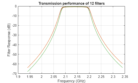
Use built-in RF Toolbox™ functions for reading a set of S-Parameter data files. For each filter plot the S21 dB values. The names of the files are AWS_Filter_1.s2p through AWS_Filter_12.s2p. These files represent 12 passband filters with similar specifications.

numfiles = 12;
filename = "AWS_Filter_"+(1:numfiles)+".s2p";    % Construct filenames
S = sparameters(filename(1));                    % Read file #1 for initial set-up
freq = S.Frequencies;                            % Frequency values are the same for all files
numfreq = numel(freq);                           % Number of frequency points
s21_data = zeros(numfreq,numfiles);              % Preallocate for speed
s21_groupdelay = zeros(numfreq,numfiles);        % Preallocate for speed

% Read Touchstone files
for n = 1:numfiles
    S = sparameters(filename(n));
    s21 = rfparam(S,2,1);
    s21_data(:,n) = s21;
    s21_groupdelay(:,n) = groupdelay(S,freq,2,1); 
end
s21_db = 20*log10(abs(s21_data));

figure
plot(freq/1e9,s21_db)
xlabel('Frequency (GHz)')
ylabel('Filter Response (dB)')
title('Transmission performance of 12 filters')
axis on
grid on

Filter Passband Visualization

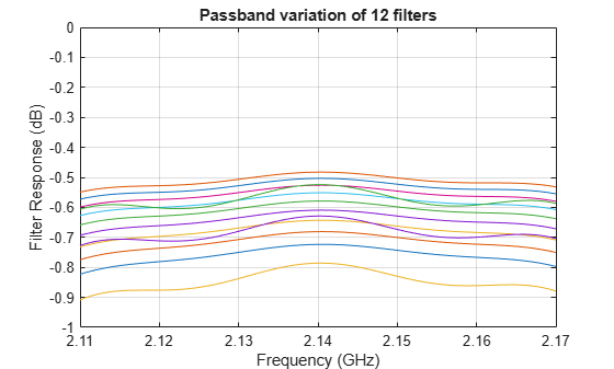
In this section, find, store, and plot the S21 data from the AWS downlink band (2.11 - 2.17 GHz).

idx = (freq >= 2.11e9) & (freq <= 2.17e9);
s21_pass_data = s21_data(idx,:);
s21_pass_db = s21_db(idx,:);
freq_pass_ghz = freq(idx)/1e9; % Normalize to GHz

plot(freq_pass_ghz,s21_pass_db)
xlabel('Frequency (GHz)')
ylabel('Filter Response (dB)')
title('Passband variation of 12 filters')
axis([min(freq_pass_ghz) max(freq_pass_ghz) -1 0])
grid on

Basic Statistical Analysis of S21 Data

To determine whether the data follows a normal distribution and if there is an outlier, perform statistical analysis on the magnitude and group delay of all passband S21 data sets.

abs_S21_pass_freq = abs(s21_pass_data);

Calculate the mean and the STD of the magnitude of the entire passband S21 data set.

mean_abs_S21 = mean(abs_S21_pass_freq,'all')

mean_abs_S21 = 0.9289

std_abs_S21 = std(abs_S21_pass_freq(:))

std_abs_S21 = 0.0104

Calculate the mean and STD of the passband magnitude response at each frequency point. This determines if the data follows a normal distribution.

mean_abs_S21_freq = mean(abs_S21_pass_freq,2);
std_abs_S21_freq = std(abs_S21_pass_freq,0,2);

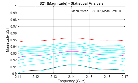
Plot all the raw passband magnitude data as a function of frequency, as well as the upper and lower limits defined by the basic statistical analysis.

plot(freq_pass_ghz,mean_abs_S21_freq,'m')
hold on
plot(freq_pass_ghz,mean_abs_S21_freq + 2*std_abs_S21_freq,'r')
plot(freq_pass_ghz,mean_abs_S21_freq - 2*std_abs_S21_freq,'k')
legend('Mean','Mean + 2*STD','Mean - 2*STD')
plot(freq_pass_ghz,abs_S21_pass_freq,'c','HandleVisibility','off')
grid on
axis([min(freq_pass_ghz) max(freq_pass_ghz) 0.9 1])
ylabel('Magnitude S21')
xlabel('Frequency (GHz)')
title('S21 (Magnitude) - Statistical Analysis')
hold off

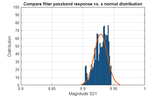
Plot a histogram for the passband magnitude data. This determines if the upper and lower limits of the data follow a normal distribution.

histfit(abs_S21_pass_freq(:))
grid on
axis([0.8 1 0 100])
xlabel('Magnitude S21')
ylabel('Distribution')
title('Compare filter passband response vs. a normal distribution')

Get the groupdelay of the passband S21 data. Use inner 60% of the bandwith for statistical analysis of the groupdelay and normalize it to 10 ns.

idx_gpd = (freq >= 2.13e9) & (freq <= 2.15e9);
freq_pass_ghz_gpd = freq(idx_gpd)/1e9; % Normalize to GHz
s21_groupdelay_pass_data = s21_groupdelay(idx_gpd,:)/10e-9; % Normalize to 10 ns

Calculate the per-frequency mean and standard deviation of the normalized group delay response. All the data is collected into a single vector for alter analysis.

mean_grpdelay_S21 = mean(s21_groupdelay_pass_data,2);
std_grpdelay_S21 = std(s21_groupdelay_pass_data,0,2);
all_grpdelay_data = reshape(s21_groupdelay_pass_data.',numel(s21_groupdelay_pass_data),1);

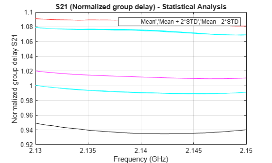
Plot all the normalized passband groupdelay data as a function of frequency, including the upper and lower limits defined by the basic statistical analysis.

plot(freq_pass_ghz_gpd,mean_grpdelay_S21,'m')
hold on
plot(freq_pass_ghz_gpd,mean_grpdelay_S21 + 2*std_grpdelay_S21,'r')
plot(freq_pass_ghz_gpd,mean_grpdelay_S21 - 2*std_grpdelay_S21,'k')
legend('Mean','Mean + 2*STD','Mean - 2*STD')
plot(freq_pass_ghz_gpd,s21_groupdelay_pass_data,'c','HandleVisibility','off')
grid on
xlim([min(freq_pass_ghz_gpd) max(freq_pass_ghz_gpd)])
ylabel('Normalized group delay S21')
xlabel('Frequency (GHz)')
title('S21 (Normalized group delay) - Statistical Analysis')
hold off

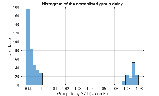
Plot a histogram for the normalized passband group delay data. This determines if the upper and lower limits of the data follow a uniform distribution.

histogram(all_grpdelay_data,35)
grid on
xlabel('Group delay S21 (seconds)')
ylabel('Distribution')
title('Histogram of the normalized group delay')

Related Topics

• Bandpass Filter Response Using RFCKT Objects
• Bandpass Filter Response

×

Open Example

You have a modified version of this example. Do you want to open this example with your edits?

No, overwrite the modified version Yes