Incorporate SGLT2 Inhibition into Physiologically Based Glucose-Insulin Model Using SimBiology Model Builder
This example shows how to add SGLT2 inhibition by a hypothetical compound to an existing glucose-insulin model using SimBiology Model Builder.
Glucose-Insulin Model
This model is another SimBiology implementation of the glucose-insulin model referenced in the Simulate the Glucose-Insulin Response example. The model is based on the publication by Dalla Man, et al. In their 2007 publication [1], the authors developed a model for the human glucose-insulin response after a meal. This model describes the dynamics of the system using ordinary differential equations. The authors used their model to simulate the glucose-insulin response after one or more meals, for normal human subjects and for human subjects with various kinds of insulin impairments.
Sodium-Glucose Cotransporter-2 (SGLT2) Inhibition
The SGLT2 receptor has been shown to facilitate around 50% of renal glucose reabsorption [3]. This example assumes to have a hypothetical SGLT2 inhibitor compound that inhibits SGLT2 by 50%. A reasonable dosing regimen and PK properties are also assumed. In this example, you incorporate the pharmacokinetics/pharmacodynamics (PK/PD) of this inhibitor compound into the glucose-insulin model.
Incorporate Inhibitor PK by Adding and Configuring Reactions
In the following steps, you model the compound absorption and clearance of a hypothetical SGLT2 inhibitor compound by using two reactions.
Load SGLT2 Model
Enter the following command to open the SimBiology Model Builder app with a prebuilt but incomplete insulin-glucose model.
openExample('simbio/SGLT2SimBiologyExample')
Add and Configure Reactions
Note
On macOS, use the command key instead of Ctrl.
Drag and drop two species blocks from the toolbar of the Diagram tab. You can place them below the annotation block Therapy, which is just a label (text) block.

Press Ctrl and drag a line from the first species to the second species. A reaction block appears in between. This reaction represents the compound absorption.
Edit the default species name by double-clicking it. Rename
species_1toGI_SGLT2_Inhibandspecies_2toPlasma_SGLT2_Inhib.
Click the reaction block. In the Property Editor pane on the right, change the reaction Name to
compound_absorption.In the Kinetic Law section, change the autocreated Forward rate parameter kf to
k_compound_absorption. The model already has the forward rate parameterk_compound_absorptionthat was created previously. The app uses green text for parameter names and blue text for species names in the reaction rate expression.Tip
To change the default reaction configurations, click Preferences on the Home tab. In the preferences dialog, click Model Building. In the Reaction Building section, there are three options to change the default kinetic law, create parameters for the kinetic law, and change the scope of created parameters.
In the States table, set the units of the two species to
milligram.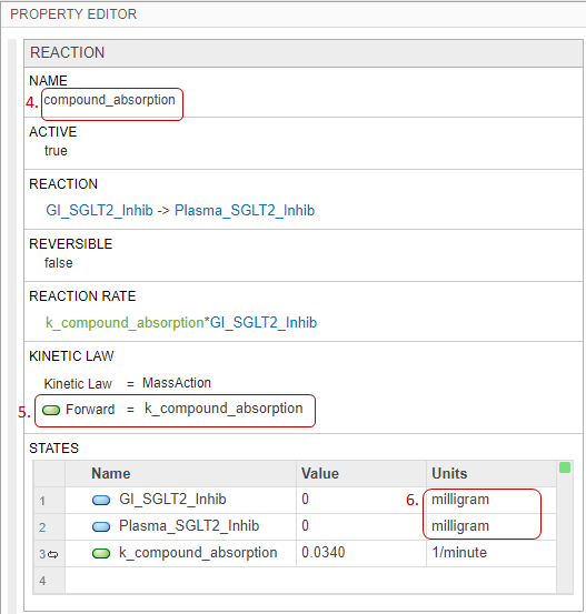
Drag and drop another reaction block from the diagram toolbar to model the compound clearance.
Press Ctrl and drag a line from
Plasma_SGLT2_Inhibto the reaction.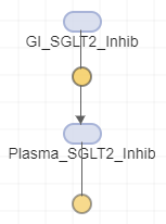
Tip
If the blocks are not aligned, you can align them using the alignment tools. On the Home tab, select Diagram Tools >
Diagram Alignment Tools.Click the reaction block. In the Property Editor pane, change the reaction Name to
compound_clearance.Update the Reaction Rate to
CL/Vd*Plasma_SGLT2_Inhib. CL and Vd indicate the model parameters for the clearance and volume of distribution, respectively.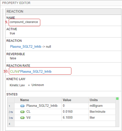
Tip
The kinetic law for a newly added reaction is configured to MassAction by default, and the SimBiology Model Builder app automatically creates and maps the species and parameters needed by the reaction rate. For other kinetic laws, only parameters are created and mapped. You need to create and map the species manually. Use the Unknown kinetic law to define a custom reaction rate with its own parameters. You must define and add the species and parameters needed by the custom rate.
The MassAction and Unknown kinetic laws can have different simulation results even when the reaction rate is the same. This can happen when you have a reversible reaction with species in different compartments. The difference in simulation results is because of the volume-scaling performed by SimBiology during the dimensional analysis. For details, see Derive ODEs from SimBiology Reactions. Specifically, for MassAction, SimBiology uses corresponding compartment volumes to multiply the forward and reverse rates. However, for Unknown and other built-in kinetic laws, SimBiology multiplies the entire rate by only one compartment which contains the reactants. To see exactly what compartment volumes are used for scaling, open the Equations tab and check the ODEs section.
Incorporate Inhibitor PD Using Mathematical Equation
SimBiology lets you define a mathematical expression to define or update the value of a model quantity during simulation. For details, see Definitions and Evaluations of Rules in SimBiology Models. In the following steps, you add a repeated assignment rule to incorporate the inhibitor pharmacodynamics by defining the renal threshold at which plasma glucose is excreted based on the compound efficacy.
In the Browser pane, click the plus icon on the browser toolbar and select
Add Repeated Assignment. The app moves the focus to the last empty row in the Repeated Assignments table.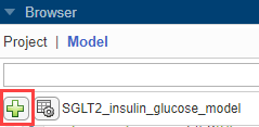
Double-click the row and enter the following expression that represents the compound inhibition based on the Hill equation:
renal_threshold =
        basal_renal_threshold*(1-compound_Imax*Whole_Body.Plasma_SGLT2_Inhib^2/(compound_IC50^2+Whole_Body.Plasma_SGLT2_Inhib^2))
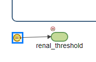
The Diagram tab now shows the repeated assignment rule block for the
renal_thresholdparameter.Tip
To view the entire model and pan through it, expand Model Assessment Tools in the Browser pane and click Overview.
Note
The app shows only a parameter block for a parameter that is on the left hand side (LHS) of a repeated assignment rule, rate rule, or event function.
The app shows only rule blocks for repeated assignments and rate rules.
The app uses dash-dot lines to connect the quantities on the right hand side of a rule. By default, these lines are not shown. To display the lines, click a rule block. From the Property Editor pane, in the Block section, set Expression Lines to show.
Update Renal Excretion Reaction to Incorporate Presence of Inhibitor Compound
The renal excretion reaction of the model is currently defined as Plasma_Glucose
-> Urinary_Glucose_Excr_AUC with the reaction rate parameter
glucose_excretion. The rate parameter is defined by a repeated assignment
rule as glucose_excretion =
(Plasma_Glucose>renal_threshold)*GFR*(Plasma_Glucose-renal_threshold), where
GFR is a glomerular filtration rate that determines the flux of the reaction
and has impact on SGLT2 inhibition effect.
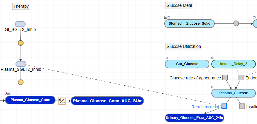
In the following steps, you update the renal excretion reaction to Plasma_Glucose
+ Plasma_SGLT2_Inhib -> Plasma_SGLT2_Inhib + Urinary_Glucose_Excr_AUC_24hr, where the
inhibitor compound Plasma_SGLT2_Inhib is both a reactant and product of the
reaction.
In the Diagram tab, click the gray square reaction block named
Renal excretion.
In the Property Editor pane, update the Reaction string to
Plasma_Glucose + Plasma_SGLT2_Inhib -> Plasma_SGLT2_Inhib + Urinary_Glucose_Excr_AUC_24hr. A dashed line now connectsPlasma_SGLT2_Inhibto the reaction block on the Diagram tab.Note
SimBiology uses a dashed line to indicate that a species is both a reactant and product of a reaction and is not being consumed by the reaction.
Split and Clone Block
When there are multiple references to the same quantity, multiple lines are connected to the block. To make the diagram clearer, you can split the block, that is, create copies of the same block, so that each reference is connected to a different copy of the block. You can also clone a block to add another use for it. For instance, you can first clone a species block to reference in multiple expressions. You can then use each clone in each expression as you build the model.
In the following steps, you clone the Plasma_SGLT2_Inhib block. These
steps are optional and do not have any effect on the model behavior.
Click the
Plasma_SGLT2_Inhibblock in the diagram.In the Property Editor pane, scroll to the Split section.
Click Clone.

In the Diagram tab, a cloned block appears next to the original block. Each block now has a clone indicator.

You can now move the dashed line to the cloned block. First click the dashed line. Press Ctrl and drag the dashed line to the cloned block. A green plus icon appears when the line is near the cloned block. Release the mouse to attach the line to the cloned block.

You can now move the cloned block closer to the
Renal excretionreaction block to make the diagram easier to read.
Incorporate Sudden Changes in Model Behavior Using Event
You can model sudden changes in model behavior based on a specified condition. For example, you can reset a species amount at a certain time point or when a certain concentration threshold is crossed. SimBiology lets you model such changes using a modeling component called an event. An event lets you specify discrete transitions in quantity values that occur when a custom condition becomes true. Such a condition is called an event trigger. Once the condition becomes true, one or more event functions are executed. For details, see Events in SimBiology Models.
In the following steps, you reset the total amount of urinary glucose to zero every 24 hours by adding one event trigger and five event functions.
Click the plus icon on the Browser toolbar. Select
Add Event. The app moves the focus to the last empty row in the Events table.Enter the following event trigger:
time >= (num_day+1)*timeDay.In the next EventFcn row, enter
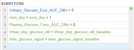
Urinary_Glucose_Excr_AUC_24hr = 0.
To add a second event function to the same event, go to the Property Editor pane of the event. In the Event Fcns table, double-click the empty row and enter the following:
num_day = num_day +
      1
.
Add three more event functions as follows:
Plasma_Glucose_Conc_AUC_24hr = 0Vmax_dep_glucose_util = Vmax_dep_glucose_util_baselinebeta_glucose_signal = beta_glucose_signal_baseline
Add Doses
SimBiology lets you model the increase in the amount of a species due to a stimulus such as
an oral or intravenous administration of a drug. To model such an increase in a species amount,
use the dose modeling component. In the following steps, you model the intake of
the inhibitor drug, such as one time per day for x numbers of days, by
dosing the GI_SGLT2_inhib species.
In the Browser pane, click the Show doses icon on the toolbar.
The Doses tab appears. In the Doses section, each row represents a dose. The Type column lets you choose between Repeat Dose (default) and Schedule Dose. The Active column lets you select which doses to apply when you simulate the model.
Double-click the Name column in the last empty row and enter
SGLT2 Inhib QD.
In the Properties section, for Target Name, enter
GI_SGLT2_Inhiband selectWhole_Body.GI_SGLT2_Inhib.In the Dose section, enter the following:
Amount =
300Rate =
0StartTime =
timeBreakfastInterval =
1440RepeatCount =
7
In the Units section, enter the following:
AmountUnits =
milligramRateUnits =
TimeUnits =
minute

Represent Biological Variability Using Variants
You can model biological variability using a modeling component called a variant. A variant is a collection of quantities with alternative values. For instance, in this example, you can have a set of parameter values for a type 2 diabetic patient and another set of values for a patient without type 2 diabetes.
For the purposes of this example, the model already has two variants. In the following steps, you open the Variants tab, where you can edit or add more variants.
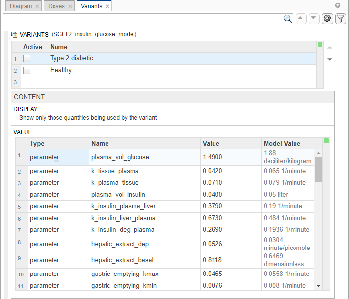
In the Browser pane, click the Show variants icon on the toolbar.
The Variants tab appears. In the Variants section, each row represents a variant. The Active column lets you select which variants to apply when you simulate the model. You can select multiple variants, and if there are duplicate specifications for a quantity value, the last occurrence for the value in the array of variants is used during simulation. The app applies the variants in the order that they appear in the table from top to bottom. Reordering the variants can change the initial conditions because the variants are applied in the new order. Make sure that you provide the correct order when you simulate the model in the Model Analyzer app. The Value column in the Content section shows the final quantity value after applying all variants that you have selected.
By default, the Content section shows only those quantities being modified by the variant. To see all model quantities, select
Show all quantities
        in the model
in the Display section.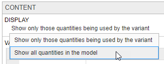
Show Model Equations and Initial Conditions
You can view the underlying system of equations, namely, ordinary differential equations (ODEs) and rules that represent the model. SimBiology derives the ODEs from model reactions, and the ODEs define what quantities to integrate during model simulation. For details, see Model Simulation.
You can use the model equations and initial conditions to debug a model. For instance, you can check the initial conditions of ODEs to see if the quantity values are initialized as you expect. You can also see how SimBiology corrects the dimensions of ODEs by dividing the right-hand-sides of equations with compartment volumes. The volume-correction information can help you debug unexpected simulation results, especially when you have a multicompartment model with different compartment volumes.
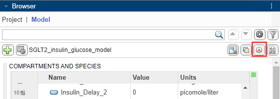
To view the model equations, click the Show model equations icon on the toolbar of the Browser pane.
![]()
The app opens the Equations tab.
Reaction Fluxes
By default, the app embeds the reaction fluxes when it displays in the model equations. Clear the Embed Fluxes check box to see the Fluxes section separately.
![]()
Generally, reaction fluxes are equivalent to reaction rates except that the dimensions of
fluxes are always amount/time. The dimensions of reaction rates can be in
concentration/time or amount/time. For details, see
Derive ODEs from SimBiology Reactions.
Initial Conditions
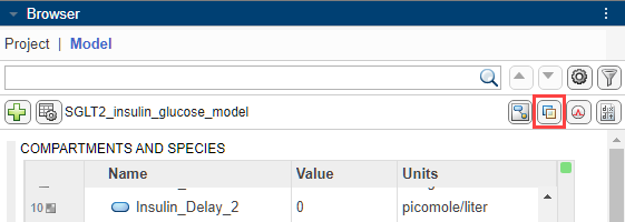
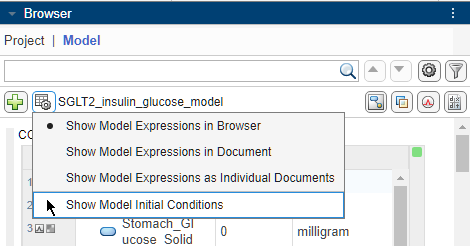
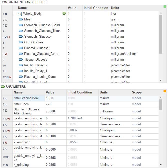
You can view the initial conditions of model quantities, namely compartments, species, and parameters. The initial conditions are the quantity values at simulation time = 0. On the toolbar of the Browser pane, select View model documents options > Show Model Initial Conditions.
The app adds a column named Initial Condition to the Compartments and Species table and Parameters table.
Define Observable Expressions
SimBiology lets you perform postsimulation calculations by defining and evaluating custom
expressions. Such an expression is called an SimBiology.Observable. In the following steps, you
add observable expressions to the model to calculate the Cmax and mean values of the
concentration-time profile of the plasma glucose.
Click the plus icon on the browser toolbar. Select
Add
       Observable
. The app moves the focus to the last empty row in the Observables table.Double-click the empty row and enter the following expression to get the Cmax value:
Cmax_plasma_glucose = max(Plasma_Glucose_Conc).
Enter the Units of the observable as
milligram/deciliterin Property Editor.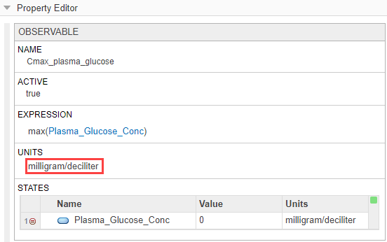
Double-click the next empty row and enter the following expression to get the mean value:
Mean_plasma_glucose = mean(Plasma_Glucose_Conc).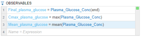
Enter the Units of the observable as
milligram/deciliterin Property Editor.
Visualize Model Behavior Using Model Simulation Tool
You can visualize the model dynamics by using the Model Simulation tool. The tool provides a convenient way to simulate the model and plot the time courses of model quantities or observables, without having to run a simulation program in the Model Analyzer app.
The Model Simulation tool is located on the right-hand side of the app
beneath the Property Editor pane. In the following steps, you plot the time
courses of the species Plasma_Glucose_Conc and
GI_SGLT2_Inhib.
Note
If you have not completed the prior model building steps, you can load the completed project instead to continue this tutorial.
Enter the following command at the command line:
openExample('simbio/SGLT2SimBiologyExample')SimBiology Model Builder opens with the incomplete SGLT2 model loaded.
Click Open and navigate to the current folder. Select the project file named
SGLT2_model.sbprojto open the completed model.
Click the arrow next to the tool name which is located below the Property Editor pane.
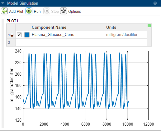
Click Add Plot on the toolbar.
Plot1 appears. Double-click the cell under Component Name and type:
Plasma_Glucose_ConcAs you type, the app provides suggestions. Select
Whole_Body.Plasma_Glucose_Conc.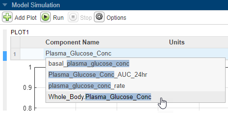
Select Options >
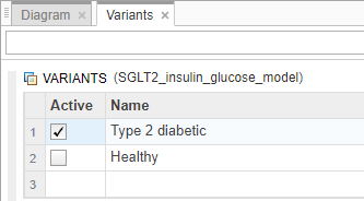
Define Active Variants for
       Simulation
. It opens the Variants tab.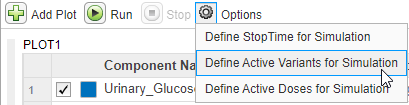
Select Type 2 diabetic in the Variants table.
Select Options >
Define Active Doses for
       Simulation
. It opens the Doses tab. Select Daily Breakfast, Daily Lunch, Daily Evening, and SGLT2 Inhib QD in the Doses table.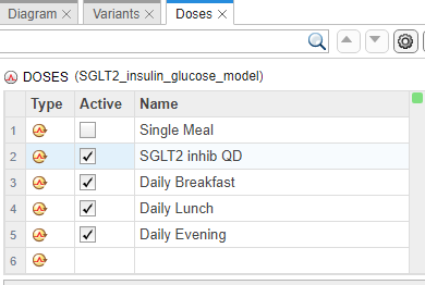
Click Run on the tool bar to see the time course of the species.
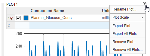
To export the plot, point the mouse to the top right corner of the table and click the options menu icon. Click Export Plot from the list.
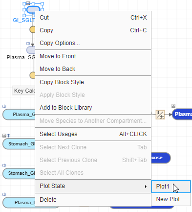
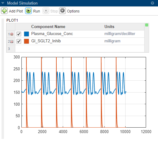
You can also use the context menu of a model quantity to add them to an existing plot or a new plot in the simulation tool. Go to the Diagram tab (or in the Browser pane), right-click the GI_SGLT2_Inhib species and select Plot State > Plot1. The species is now added to the plot.
Click Run again to update the plot.
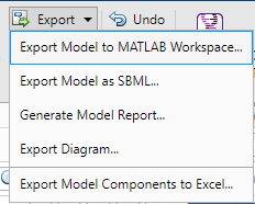
Export Model
SimBiology Model Builder lets you export the model to various file formats. You can:
Export the model to the MATLAB workspace. Once the model is in the workspace, you can work on it programmatically. For more command-line examples, see Build and Verify Models.
Export the model to an SBML file.
Generate a model report that summarizes the various details of the model.
Export just the model diagram.
Export the model components to Excel® files.
On the Home tab, in the Model section, select Export.
Tip
If you have previously open the example, you can find the completed model in
SGLT2_model.sbproj which is located in a subfolder of the current running
release Examples folder.
References
[1] Dalla Man, Chiara, Robert A. Rizza, and Claudio Cobelli. “Meal Simulation Model of the Glucose-Insulin System.” IEEE Transactions on Biomedical Engineering 54, no. 10 (October 2007): 1740–49. https://ieeexplore.ieee.org/document/4303268.
[2] Dalla Man, Chiara, M. Camilleri, and C. Cobelli. “A System Model of Oral Glucose Absorption: Validation on Gold Standard Data.” IEEE Transactions on Biomedical Engineering 53, no. 12 (December 2006): 2472–78. https://ieeexplore.ieee.org/document/4015600.
[3] Wright, Ernest M., Donald D. F. Loo, and Bruce A. Hirayama. “Biology of Human Sodium Glucose Transporters.” Physiological Reviews 91, no. 2 (April 2011): 733–94. https://journals.physiology.org/doi/full/10.1152/physrev.00055.2009.
See Also
SimBiology Model Analyzer | SimBiology Model Builder