Foundation Library
Error diagnostics in block dialog boxes
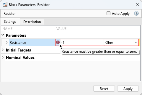
When you enter an invalid parameter value that would trigger an assert and result in a compile-time error, in many cases, you can now immediately see the error in the block dialog box or Property Inspector. For example, if you enter a negative value for the Resistance parameter, the block dialog box displays a red exclamation point next to the parameter name. To view the error message, pause the cursor over the exclamation point.
New angle-based and position-based blocks
To extend angle-based and position-based modeling capabilities, these blocks have been added to the Mechanisms library:
Additionally, the Translational Inerter (PB) block has been added to the Translational library.
Phase-Change Thermal Mass block
The new Phase-Change Thermal Mass block represents a mass of two-phase material in a thermal network. Use this block to model ice storage air conditioners or systems that use the phase-change materials in electronics and battery cooling applications.
Model gas or moist air reservoirs using total pressure and temperature
The Reservoir (G) and Reservoir (MA) blocks have a new parameter, Reservoir specification, that allows you to choose between two modeling options:
Static pressure and static temperature— Specify pressure and temperature as boundary conditions at the reservoir port. Use this option for applications with low-speed compressible flow, such as HVAC systems. You can also use it to simulate a portion of a system based on measured pressure and temperature at the boundary. This option is equivalent to the block functionality in previous releases.Total pressure and total temperature— Specify pressure and temperature of fluid at rest inside the reservoir. As the fluid speeds up toward the exit port, its movement results in a reduction in pressure and temperature. Use this option for applications with high-speed compressible flows, such as in aerospace models, or for fluid dynamics analysis.
Additionally, some of the existing block parameter names have been shortened. To improve consistency, these parameter name changes have been implemented for the reservoir blocks in all the fluid domains:
Reservoir pressure specification is now Pressure specification.
Reservoir temperature specification is now Temperature specification.
Reservoir humidity specification is now Humidity specification.
Reservoir trace gas specification is now Trace gas specification.
Reservoir energy specification is now Energy specification.
This parameter renaming has no effect on block functionality.
Variable Gap Capacitor block
The Variable Gap Capacitor block has been added to the Foundation library. Previously, this block was part of the Simscape™ Electrical™ libraries.
Flow Rate Source (MA) and Flow Rate Sensor (MA) blocks let you specify humidity and trace gas amounts at standard conditions
When calculating volumetric flow rate by using density at standard conditions, the Flow Rate Source (MA) and Flow Rate Sensor (MA) blocks now provide a full range of humidity and trace gas parameterization options. Previously, these blocks allowed you to specify relative humidity only and assumed zero trace gas at standard conditions.
Moisture & Trace Gas Sensor (MA) block lets you specify relative humidity at saturation
The Moisture & Trace Gas Sensor (MA) block now has the Relative humidity at saturation parameter, which lets you specify a value for relative humidity at saturation when measuring wet-bulb temperature. Previously, the block always assumed relative humidity at saturation to be 1.
Spectrum Analyzer Block: Streamlined user interface, new print-to-figure option, and updated status bar readouts
The Spectrum Analyzer block includes the following enhancements in R2026b.
Streamlined user interface
The Spectrum Analyzer toolstrip has been reorganized into these three tabs to provide easy and streamlined access to the scope settings:
Home tab contains all the general settings for spectrum and spectrogram display.
Estimation tab contains settings that control frequency resolution and spectral averaging.
Measurements tab contains settings to control the various measurements supported by the scope.
New print-to-figure option
Print the Spectrum Analyzer scope display to a MATLAB® figure by clicking the Print to Figure option in the Home tab > Export section.
Updated status bar readouts
Certain parameter names in the spectrum analyzer status bar have changed. Some of these parameters have new readouts. For more information, see the following table.
| Status Bar Parameter In R2026a or Earlier | Status Bar Parameter In R2026b | Status Bar Readout In R2026b |
|---|---|---|
Sample Rate
|
Sample Rate (Fs)
|
Fs
|
Samples/Update
|
Samples/Update (S/U)
|
S/U
|
Time Resolution
|
Time Resolution (ΔT)
|
ΔT
|
NFFT
|
FFT Length (NFFT)
|
NFFT
|
Forgetting Factor
|
Forgetting Factor (α)
|
α
|
Spectral Averages
|
Spectral Averages (Navg)
|
Navg
|
Part Repository: Include metadata with part list
When you use the partrepo.collection.listDataSetsForBlock function to list the available
parts for a Simscape block, the function now also includes the associated metadata in the
table for each part.
Block Icon Editor Enhancement: Inherit domain styles for Simscape block icons
You can use the Inherit styles option in the
Format section of the Icon Editor to make elements of
the block icon inherit port domain styles. For example, in a Variable
Resistor block icon, to make an arrow through the rectangle inherit the
style based on the left-side input port, select the arrow and set Inherit styles to L0 : Input.
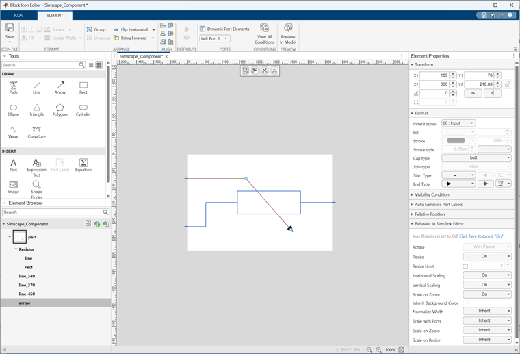
For more information, see Icon Editor.
Functionality being removed or changed
Hydraulic block library and domain have been removed
The Hydraulic block library and domain have been removed. If you open a model that contains Hydraulic library blocks or custom blocks that use the hydraulic domain, the model displays an error. Use the Isothermal Liquid library and domain instead.
Flow Resistance (G) block uses inlet density instead of average density
Behavior change
To improve consistency between the moist air and gas domains, the Flow Resistance (G) block now calculates the flow rate by using the inlet density, instead of the average density. This change can produce a small difference in simulation results, compared to the previous releases.
Using external signals to limit PS Integrator block output generates an error
Errors
If your model contains a PS Integrator block with the Limit output source
parameter set to External, you get a compile-time error.
Set Limit output source to Internal
and use the Upper limit and Lower limit
parameters to define the saturation bounds.
Simulation
Energy Accounting: Use data logging to get energy and power usage for specified block
You can get energy and power usage for Simscape blocks in your model by enabling energy accounting. In the Configuration Parameters dialog box, at the bottom of the Simscape pane, under Advanced Parameters, select the Enable energy accounting check box.
You can also use the equivalent command-line interface to set the model configuration parameter:
set_param(bdroot,"SimscapeUseEnergyAccounting","on")
Energy accounting is based on post-processing logged simulation data. Enable Simscape data logging for either the whole model or for individual blocks, then
simulate the model. You can then use the new getEnergyInfo function to get the energy and power usage for a specified
block.
Partitioning Solver: New partitioning methods
You can now set the Partitioning method parameter in the Solver Configuration block to one of these updated options:
Stable simulation (maximize stability)— Improve simulation robustness by maximizing the use of implicit solvers for groups of equations.Balanced simulation (balance nonlinearities and stability)— Balance speed and robustness by increasing the use of implicit solvers for groups of equations.Fast simulation (minimize nonlinearities)— Improve simulation performance by maximizing the use of explicit solvers for groups of equations.
The Robust simulation option has been renamed to
Balanced simulation (balance nonlinearities and stability).
Simscape updates models from prior versions to use the new option.
Trapezoidal Solver: Multicore function evaluation
To apply multithread function evaluation when using the trapezoidal solver in the
Solver Configuration block, set
Solver type to Trapezoidal Rule, and
set Maximum threads for function evaluation to a value greater than
1.
Simscape Initialization Analyzer: Interface enhancements
You can now open the Simscape Initialization Analyzer app from the Apps tab in the Simulink® toolstrip. The app gives you the new option to filter Simscape variables by name.
Enabled Subsystems: Reset states to initial conditions
When you use an Enabled Subsystem block in a Simscape model, you can now set States when enabling to
reset. To reset the subsystem states to their initial
conditions, disable the subsystem for at least one time step.
Run-Time Parameters: Update with Reinitialize Function block or Enabled Subsystem block
You can now use the Reinitialize
Function block or the reset option of an Enabled Subsystem block to update run-time parameters.
Run-Time Parameters: Update workspace variables or mask parameters used by run-time parameters using Parameter Writer block
Starting in R2026b, you can use the Parameter Writer block to update base workspace variables, model workspace variables, mask parameters, and Simulink data dictionary variables used by the run-time parameters of Simscape blocks. This capability expands the scope of the Parameter Writer block beyond Simulink blocks.
Large-Model Compilation: Disk caching performance improvements
Disk caching of model compilation artifacts, introduced in R2024b, improves the performance of the first compilation of a model in a given session. However, subsequent compilations using disk caching could be slower than with memory caching. The first compilation after switching between disk and memory caching within a given session was also slower. In R2026b, multiple enhancements in the areas of incremental compilation and disk caching result in faster compilation of large models. The table shows improved compilation speeds for three example models.
| Example Model | First Compile after Switching from Disk to Memory Caching | First Compile after Switching from Memory to Disk Caching | Subsequent Compiles with Disk Caching |
|---|---|---|---|
| Electric Vehicle Thermal Management with Heat Pump (Simscape Fluids) | R2026a: 26.718 s R2026b: 22.374 s | R2026a: 29.124 s R2026b: 25.007 s | R2026a: 18.508 s R2026b: 17.830 s |
| Battery Pack DC Fast Charging (Simscape Electrical) | R2026a: 42.785 s R2026b: 36.792 s | R2026a: 44.614 s R2026b: 38.791 s | R2026a: 22.913 s R2026b: 21.771 s |
| Model High-Voltage Direct-Current Transmission Using Modular Multilevel Converters (Simscape Electrical) | R2026a: 12.084 s R2026b: 7.505 s | R2026a: 12.520 s R2026b: 8.471 s | R2026a: 7.401 s R2026b: 6.953 s |
These results were obtained on a Windows® 11, Intel® CPU i9-13900K @ 3.00 GHz with SSD read/write speeds of 7,000 MB/s and 5,800 MB/s, respectively.
For more information on disk caching, see Disk Caching of Compilation Artifacts.
Simscape-to-HDL Enhancements: New and improved motor models
When you use Simscape-to-HDL code generation, you can now:
Automatically replace Simscape motors with optimized equivalents for FPGA deployment.
Take advantage of improved position handling for PMSM blocks in long-running simulations.
To learn more about R2026b Simscape-to-HDL features, see Release Notes for HDL Coder (HDL Coder).
Functionality being removed or changed
Data streaming to Simulation Data Inspector has been removed
The Record data in Simulation Data Inspector configuration parameter, which enabled streaming of logged Simscape simulation data directly to Simulation Data Inspector, has been removed. Use the Instrumentation table and selective data logging instead. For more information, see About Selective Logging.
If you open an existing model that used to stream Simscape data directly to the Simulation Data Inspector, the model now logs data either to memory or to disk, depending on its Stream data to temporary disk directory setting. For more information, see Saving and Retrieving Logged Simulation Data.
To visualise the logged Simscape simulation data in the Simulation Data Inspector, use the
Simulink.sdi.createRun function and
import the data as a workspace variable. You can use this syntax, where
simlog is a simscape.logging.Node object:
Simulink.sdi.createRun(runName,"vars",simlog)
Simscape Language
Remove zero crossings from Simscape Language expressions
You can remove the zero crossings caused by functions, relational operators, and operators in
Simscape Language expressions by using the nozc
Use identity matrices in equations
You can now use the eye function to create and use identity
matrices in the equations section and in
simscape.Value objects.
For a complete list of functions supported in the
equations section, see Supported Functions.
Functionality being removed or changed
setup section will be removed
Warns
If your file contains a setup section, the
compiler issues a warning that it will be removed in a future release. Using
setup can cause issues with configuring run-time
parameters. It also has negative impact on compilation performance.
Other constructs available in the Simscape language let you achieve the same results without compromising compilation performance and run-time capabilities.
| Task | Recommended Technique |
|---|---|
Validate parameters | Use an |
Compute derived parameters | Use Simscape functions or declaration functions. For more information, see Simscape Functions and Declaration Functions. |
Set initial conditions | Assign variable priority and target value. For more information, see Variable Priority for Model Initialization. |
Designate source for domain parameters | Use direct assignment to a domain parameter in the component node declaration. For more information, see Source Components. |
Improved error checking for case-sensitivity and non-ASCII characters in file names and member declarations
Behavior change
Stricter error checking has been implemented with respect to case-sensitivity of class and member declarations. In previous releases, sometimes the case mismatch between a member declaration in a composite component and the actual domain or component name did not result in an error. Starting in R2026a, if there is a case mismatch, the compiler generates an error. To help you resolve the case mismatch, the error message contains the name of the file on the MATLAB path.
Similarly, sometimes invalid text characters at the end of file or member names were treated as comments. Error checking for invalid characters has now been improved. If you get an error message about invalid text character, check your code for an unsupported symbol, invisible character, or unintentional copy-pasting of non-ASCII characters.
Thermal liquid domain parameter values have been adjusted
Behavior change
The parameter values of the thermal liquid domain definition have been updated to include the addition of entrained air. These changes match the changes to the default parameter values of the Thermal Liquid Settings (TL) block. For more information, see the Version History section of the Thermal Liquid Settings (TL) block.
Foundation Library
Part Data Sets: Author and install part collections
You can now build, share, and install collections of parts. Collections can hold multiple parts for multiple blocks in an MLDATX file. When you install a collection, the parts in that collection are available to parameterize blocks from the Block Parameterization Manager. Installing a collection does not expose the files used to create the collection.
To learn more, see Programmatically Manage Simscape Block Parameter Data.
Mechanical Angle-Based Rotational Domain and Block Library: Use angle-based modeling framework to model mechanical rotational systems
Use the new angle-based rotational domain and the Rotational block library to model mechanical rotational systems where it is important to know the component angular positions, such as mechanisms with camshafts, multiple springs, or rotational irregularities. The Rotational block library contains basic building blocks, such as inertia, spring, and damper blocks, as well as sources and sensors. The Utilities sublibrary contains the Interface (AB-Rotational) block, which allows connections between angle-based and non-angle-based mechanical rotational ports.
The new Mechanisms library contains blocks that combine angle-based rotational and position-based translational modeling principles to represent simple mechanisms, such as a cam and follower or a wheel and axle.
For more information, see Angle-Based Rotational Systems and the block reference pages. Also see Mechanical Angle-Based Rotational Domain for information about the new domain definition.
To maintain consistency between translational and rotational domains, the Translational Initial Spacer (PB) block has been renamed to Initial Length (PB). The block functionality is unchanged. Additionally, parameter and variable names of several other blocks in the Translational library have slight modifications, to match the new blocks in the Rotational library. For more information, see the block reference pages.
These changes have no compatibility impact when you use these Foundation library blocks in your models. When you open an existing model, the block and parameter names update automatically, and the parameter values and simulation results are unchanged. However, if you use these blocks in your custom composite components, you must update the composite component code.
Model position-based valves and linear actuators by using the Translational Mechanical Converter (IL-PB) block
The new Translational Mechanical Converter (IL-PB) block, in the Isothermal Liquid/Elements library, provides an interface between isothermal liquid and position-based mechanical translational networks. Use this block to model position-based valves and linear actuators.
Thermal liquid domain now models entrained air
The thermal liquid domain now models entrained air in the fluid flow, which is a small amount of nondissolved gas trapped in the fluid. Entrained air makes the fluid more compressible, which can reduce numerical stiffness. You can also optionally model air dissolution to allow entrained air to dissolve into the liquid.
To control the entrained air characteristics, use the Volumetric fraction of entrained air in mixture at atmospheric conditions and Specific gas constant parameters in the Thermal Liquid Properties (TL) (Simscape Fluids) or Thermal Liquid Settings (TL) blocks. To model air dissolution, select Model air dissolution.
This change has no compatibility impact to existing models that contain a Thermal Liquid Properties (TL) or Thermal Liquid Settings (TL) block. In existing models that do not include these blocks, simulation results may change because, in the absence of these blocks, the model uses the default domain parameters, which now account for entrained air effects.
Calculate fluid properties for thermal liquid models
Use the new fluidPropertiesThermalLiquid function to calculate thermal liquid property
values based on the fluid pressure and temperature.
Calculate refrigerant charge properties for two-phase fluid models
Calculate the fluid states for two-phase fluid models based on the refrigerant charge density
and temperature by using the new refrigerantChargeProperties function. Use this function to initialize
two-phase fluid models based on refrigerant charge density.
Transport properties sensors
Measure dynamic and kinematic viscosity, thermal conductivity, and Prandtl number by using these new blocks:
Additionally, the Liquid Properties Sensor (IL) block now has optional ports that measure dynamic and kinematic viscosity.
Reservoir blocks use consistent options across fluid domains
The reservoir blocks in the gas, thermal liquid, and two-phase fluid domains have been reconfigured to improve block usability and consistency across the domains:
The Controlled Reservoir (G) and Reservoir (G) blocks have been combined into the Reservoir (G) block. You specify the reservoir pressure and temperature by using block parameter values or physical signals.
The Controlled Reservoir (TL) and Reservoir (TL) blocks have been combined into the Reservoir (TL) block. You specify the reservoir pressure and temperature by using block parameter values or physical signals.
The Controlled Reservoir (2P) and Reservoir (2P) blocks have been combined into the Reservoir (2P) block. You specify the reservoir pressure and specific internal energy by using block parameter values or physical signals.
These changes are similar to the change implemented for the reservoirs in the moist air domain in R2024b.
In the isothermal liquid domain, the Reservoir (IL) block has always provided the ability to specify either constant or time-varying pressure inside the reservoir. To improve consistency with other domains, the Reservoir type parameter has been replaced with the Provide input signal for pressure check box and the block icon has changed. The block functionality is unchanged.
These changes have no compatibility impact when you use these Foundation library blocks in your models. When you open an existing model, the reservoir blocks update automatically. However, if you use controlled reservoir blocks in your custom composite components, you must update the composite component code.
Thermal Resistor block enhancements
For most applications, you define the thermal behavior of the block by specifying the dissipation factor and thermal time constant. The product of these two quantities is the thermal mass of the resistor. In certain applications, it is more convenient to define the thermal mass as a product of mass and specific heat capacity of the resistor. Use the new Thermal mass parameterization parameter to select between these two parameterization methods:
Specify time constant and dissipation factor— Use the product of thermal time constant and dissipation factor. This method is the same as in previous releases.Specify mass and specific heat capacity— Use the product of mass and specific heat capacity. This method is convenient when you intend to use the block as a resistive heating element.
Additionally, because some semiconductors and alloys have a negative value for the temperature coefficient of electrical resistance, you can now specify negative values for the Temperature coefficient parameter.
Dynamic block icons for blocks in Physical Signals library
Several blocks in the Physical Signals library now display the parameter values on the
block icon. For example, for this PS Gain block, the value
of the Gain parameter is 1. The block displays
this value on the block icon:

The updated blocks are:
PS Bias
PS Constant
PS Gain
PS Integrator
PS Math Function
PS Transfer Function
Additionally:
The PS Step block icon flips if the Initial value is greater than the Final value.

The PS Ramp block icon reflects whether the Slope value is positive or negative.

Name-Based Port Connections: Programmatically remove and reroute connection lines between Simscape block ports
You can now programmatically remove and reroute connection lines between physical modeling ports by using the port names. Supported block types include:
Simscape blocks in the Foundation, Utilities, and add-on product libraries
Simscape Multibody™ blocks
Subsystems that contain Simscape or Simscape Multibody blocks
For more information, see simscape.removeConnection and simscape.connectedPorts.
Additionally, when you load a model saved in R2026a or in a later release, connections between blocks are mapped based on port names, not on port positions on the left or right side of the block, as before. Models saved in earlier releases continue to use port positions for mapping connections.
This enhancement increases the model robustness by preserving the connections in existing models if a library block icon is modified or rotated. This change has no compatibility impact. However, if you use custom block libraries where the library author changes the port side in or after R2026a, connections in models saved before R2026a may be broken or incorrect.
If the port configuration of a custom library block has been changed in a way that results in broken connections when you load a model saved in a previous release, you get a warning with a link to the block that broke the connections. Clicking this link highlights the block in the model.
Context menu usability improvements
In R2026a, the context menus that appear when you right-click an object on the model canvas have changed. For example, this image shows the differences between the context menu that opens when you right-click a DC Voltage Source block in R2025b and in R2026a.
| R2025b | R2026a |
|---|---|
|
|
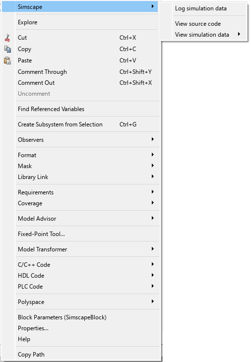
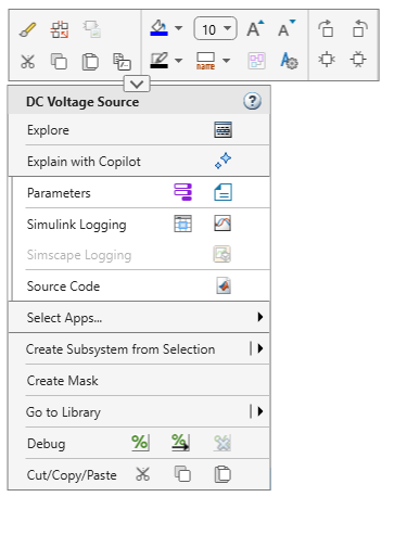
Context menu items specific to Simscape blocks include:
Simulink Logging, which contains buttons to open the Instrumentation Table and the Simulation Data Inspector.
Simscape Logging, which contains a button to open the Simscape Results Explorer. To enable this button, simulate the model with Simscape data logging turned on. You can configure Simscape data logging by using the Simscape Block tab of the model toolstrip or the Configuration Parameters dialog box. For more information, see Enable Simscape Data Logging for the Whole Model.
Source Code contains a push button to view the block source code. This option is available only for open-source blocks authored in Simscape language.
Create Mask lets you create mask-on-link for the block. Once you create the mask, Edit Mask and related options become available.
In general, these options and buttons are consistent with what appears on the Simscape Block tab of the model toolstrip. To improve this consistency, the Simscape Block tab of the model toolstrip now also has a Mask subsection, with the Create Mask and other related options. The options work the same as in the new context menu.
Additionally, data visualization options have moved from the context menu to the block dialog box. For example, to plot the fluid properties of an isothermal liquid, instead of right-clicking the Isothermal Liquid Properties (IL) block and selecting Foundation Library > Plot Fluid Properties from the context menu, you now open the block dialog box and, under Plots, click the Plot button next to Isothermal liquid properties.
When you right-click a physical connection line, the context menu contains the Trace Connections and Remove Trace options. These options are similar to the Trace Signal options for Simulink signals.
For more information on context-sensitive menu redesign and the options and buttons common to all blocks, see New Simulink context menus prioritize frequently used functionality in the Simulink Release Notes.
Affine units limitation removed
In previous releases, physical signal unit propagation did not include special
handling for affine units. Therefore, if a block specified an affine unit for its
parameter that eventually defined the untyped unit of a physical signal, the model
compilation failed because input and output signals cannot use affine units. This
limitation effectively prevented you from using affine units, such as
degC, in Physical Signal library blocks.
Starting in R2026a, if a block parameter uses an affine unit, then physical signal
unit propagation converts this unit into its fundamental unit. The conversion type is
defined by the Conversion attribute specified in the component file.
Physical Signal library blocks use the default Conversion attribute,
which is absolute.
In other words, if a block parameter specifies the unit as degC or
degF, unit propagation converts it into K as an
absolute temperature. If the model uses degC or degF
to specify a relative temperature, unit propagation yields results that are numerically
incorrect. Use deltadegC or deltadegF to specify
relative temperatures.
Spectrum Analyzer Block: Autoscaling of yaxis limits
You can now automatically scale the y-axis limits of the spectrum analyzer display by selecting the Automatically Scale Axes Limits parameter. If you clear this parameter, use the Y-Limits parameter to manually scale the axes limits.
For more information, see Spectrum Analyzer.
Functionality being removed or changed
Using external signals to limit PS Integrator block output will be removed
Warns
Currently, the PS Integrator block has the Limit output source parameter, which controls whether to specify saturation bounds as block parameters or input signals.
The ability to define the saturation bounds by using the external physical signals
at ports U and L will be removed in a future
release. Instead, set Limit output source to
Internal and use the Upper limit and
Lower limit parameters to define the saturation bounds.
Simulation
Simscape Initialization Analyzer: Analyze solver initialization performance for debugging
You can use the Simscape Initialization Analyzer app to analyze solver performance during transient initialization. Use the app to debug initialization warnings and errors or improve initialization speed for a given Solver Configuration block in a Simscape model. The app displays each solver state and plots the state when you select it. The Suggestions pane shows suggestions to improve initialization.
To open the app, enter:
simscapeInitializationAnalyzer
Descriptor State Space: Linearize Simscape models in DSS format
When you use the linearize function on a Simscape model that
contains a Descriptor
State-Space block with the Linearize to sparse model
parameter selected, both the Simulink and Simscape networks linearize using DSS format.
To learn more, see Linearize Sparse Models (Simulink Control Design).
Scalable Compilation: Automatically designate reusable components
Use the new model configuration parameter, Automatically select reusable components, to automatically select reusable components for scalable and incremental compilation. To enable this parameter, select the Reuse components during compilation model configuration parameter.
You can also use the equivalent command-line interface:
set_param(bdroot,"SimscapeAutoSelectReusableComponents","on")
The new parameter simplifies the process of configuring a model for scalable and
incremental compilation. When Automatically select reusable components
is on, the software automatically identifies appropriate reusable components and subsystems
during compilation and marks them as reusable. This automatic selection process respects the
explicit designations made by setting the simscape.reuse.setConfig
parameter or the CompileReuse attribute. If you explicitly designate
components as reusable, they continue to be treated as reusable, in addition to the
automatically selected ones. When you enable automatic selection of reusable components, you
can use sscScalableAdvisor to see which components and subsystems have been selected
as reusable.
To avoid backward compatibility issues, for existing models where Reuse components during compilation is on, the default value of the Automatically select reusable components parameter is off. For new models, as well as for existing models not currently using scalable and incremental compilation, once you select Reuse components during compilation, the Automatically select reusable components is on by default.
Enhanced discrete state naming for working with Simulink initialization and operating points
Discrete states originating from Simscape blocks now contain the state name and its block origin. You can use this
initial state information to specify initial block state values for simulation or to provide
an initial condition for linearization. For more information, see Simulink.BlockDiagram.getInitialState.
Simscape-to-HDL Enhancements
When you use Simscape-to-HDL code generation, you can now:
Tune parameter values for dynamic switches.
Generate optimized state-space data for Linear Time-Invariant (LTI) models with the Simscape HDL Workflow Advisor.
Generate code for the PWM Generator (Three-phase, Two-level) (Simscape Electrical) block.
Reduce CPU overloads by automating CPU and FPGA rate transitions.
Use fixed-point data type precision for the optimized PMSM blocks in your HDL implementation models.
To learn more about R2026a Simscape-to-HDL features, see Release Notes for HDL Coder (HDL Coder).
Add-On License Management Enhancement: Modify any parameters when working in Restricted mode
You can now modify any block parameters when working in Restricted mode. In previous releases, you could change numerical parameter values, but were not able to change drop-down values, such as the block parameterization options. This restriction has now been removed.
New examples
Examples introduced in this version include:
Additionally, angle-based rotational examples, introduced in R2025a, have been restructured and expanded. These examples now use blocks from the new Rotational library, rather than custom blocks. For more information, see Angle-Based Rotational Systems
Functionality being removed or changed
Robust ordering of variables and equations during compilation
Behavior change
Starting in R2026a, new models use the robust variable and equation ordering algorithm during compilation. This method reduces the sensitivity of the model compilation process to block and variable naming, improving the consistency of simulation results.
If you open a model created prior to R2026a, by default it uses the same variable and equation ordering method as before, and the simulation results do not change.
To upgrade your existing models to use the new algorithm, run the Check Simscape use of robust variable and equation ordering check in the Upgrade Advisor.
Data streaming to Simulation Data Inspector will be removed
Warns
The Record data in Simulation Data Inspector configuration parameter, which enables streaming of logged Simscape simulation data directly to Simulation Data Inspector, will be removed in a future release. Use the Instrumentation table and selective data logging instead. For more information, see About Selective Logging.
Option name change for simscape.op.create function
argument
Behavior change
Prestart option for the simPhase argument
has been renamed to Target. The behavior remains the same. To
learn more, see simscape.op.create.
Quality and stability improvements
R2025b delivers quality and stability improvements, building on the new features introduced in R2025a.
Simscape Language
Declare composite domains
You can now declare a composite domain as a hierarchy of other, primitive or composite, domains. A primitive domain is a regular Foundation or custom domain that has nodes of a single type: electrical, gas, and so on. A composite domain is a textual equivalent of a bus port on a rigid Simscape Bus block. Composite domains have nodes that represent a bundle of connections, possibly of different types. For example, this composite domain combines two primitive domain types: mechanical translational and electrical.
domain MechElec
% Mechanical Translational and Electrical Domain
    nodes
        m = foundation.mechanical.translational.translational;
        e = foundation.electrical.electrical;
    end
end
To use a composite domain, design composite components with external ports that belong to that domain type. Connect these components to each other and to Simscape Bus or Connection Port blocks with corresponding rigid interfaces. For more information, see Composite Domains.
Use inverse hyperbolic functions in equations
You can now use these functions in the equations
section and in simscape.Value objects:
acosh— Inverse hyperbolic cosine.asinh— Inverse hyperbolic sine.atanh— Inverse hyperbolic tangent.
For a complete list of functions supported in the
equations section, see Supported Functions.
Foundation Library
Array Connection Block: Concatenate arrays of conserving connections into single array-of-nodes port
The new Array Connection block concatenates arrays of conserving connections into a single array-of-nodes (AON) port. Use the Array Connection blocks to connect individual elements, or subsets of elements, of AON ports of different sizes. You can also use this block to declutter a model diagram by bundling multiple connections of the same type and having two Array Connection blocks, facing each other, with their AON ports connected.
Probe Block: Probe across subsystem boundaries
The Probe block now has a dialog box, which you can use to connect the Probe block to another Simscape block, select which variables to probe, and customize the Probe port names and the output units for the variables.
In previous releases, the binding process involved double-clicking the Probe block and then clicking another block on the model canvas, and therefore you could connect the Probe block only to a block at the same level of the model hierarchy. Now, when you double-click a Probe block, its dialog box opens. Use the Connect button to attach (bind) the Probe block to another Simscape block, which can be located in a subsystem, or at any other level of the model hierarchy. Once you select the block, a list of its variables appears on the model canvas, as before. You can select the variables on the model canvas, or skip this step. Click Done connecting to complete the binding process. At this point, the Probe dialog box is populated with the list of variables from the attached block. If you selected any of the variables on the model canvas, they are selected in the dialog box as well. You can use the dialog box to continue selecting which variables to probe, customize the port names, and specify the output units, the same way as in the Property Inspector. The Property Inspector workflow, introduced in R2024b, and the process of selecting the variables directly on the model canvas work the same, as before.
During the binding process, when you navigate across the subsystem boundaries to a subsystem that is not open in a model tab, the Probe block dialog box can close automatically. In this case, you can end the binding process by clicking the X in the upper-right corner of the model canvas.
Cap (IL) Block: Terminate unused isothermal liquid ports
Use the new Cap (IL) block to terminate isothermal liquid ports on other blocks or to set the initial pressure at a node.
PS State-Space Block: Implement time-invariant linear state-space system
The new PS State-Space block, in the Physical Signals/Linear Operators library, implements a state-space representation of the linear time-invariant system.
Optional zero-crossings for Physical Signals library blocks
These blocks in the Physical Signals library now have an option to disable zero-crossing detection during simulation:
This change has no compatibility impact. By default, these blocks perform zero-crossing detection, like in previous releases. To improve simulation speed, you can disable zero-crossing detection for a block by clearing the Enable zero-crossing detection check box.
Optionally model dynamic compressibility and fluid inertia in Gas pipes
The Pipe (G) block has new options for modeling gas dynamics and fluid inertia:
Enable dynamic compressibility — Select whether to account for the dynamic compressibility of gas. Dynamic compressibility gives the gas density a dependence on pressure, impacting the transient response of the system at small time scales. Disable dynamic compressibility if you want to reach steady state quickly during simulation or to simplify model initialization. By default, the block models dynamic compressibility, which is the same behavior as in previous releases.
Enable fluid inertia — Select whether to account for the gas flow inertia. Flow inertia provides resistance to changes in mass flow rate. By default, the block does not model flow inertia, which is the same behavior as in previous releases. To enable the Enable fluid inertia check box, select the Enable dynamic compressibility check box.
Additionally, the block parameterization options have changed. Instead of specifying initial targets for block variables, you now specify initial parameter values and priorities in the Effects and Initial Conditions section.
To improve consistency, the names of the existing check boxes for modeling fluid compressibility and inertia in other Fluids domains have also changed to Enable dynamic compressibility and Enable fluid inertia.
Model ideal mutual inductor with no fast pole
The Mutual Inductor block has a new
option that lets you model an ideal mutual inductor. If you select the Perfect
coupling – no leakage checkbox, the block sets the coefficient of coupling to
1 and the leakage reluctances to 0. The block
represents the ideal mutual inductor with no leakages and no fast pole, while also
retaining the correct low-frequency behavior and blocking DC.
Spectrum Analyzer Block: Control plot type and use running averaging method
You can now individually control the type of plot for each line in the Spectrum Analyzer block. Select the line and set the Plot Type accordingly.
In R2025a, the Spectrum Analyzer block supports the running averaging
method to compute the power spectrum estimate. To enable this mode, set the
Averaging Method parameter to Running
and the Spectral Averages parameter to a positive integer. For more
information, see the Algorithms section in the Spectrum Analyzer block reference page.
Use the Graph Data Extractor app to import data sheet graphs into MATLAB data files
The Graph Importer, introduced in R2024b, has been renamed the Graph
Data Extractor. You can now access the Graph Data
Extractor app from the Simscape section of the app library or
by entering graphDataExtractor at the MATLAB command prompt. Use the app to import graphs from part data sheet PDFs,
modify the point data, and then export the selected data as MATLAB data files. You can then use these data files to parameterize blocks.
To improve usability, the Graph Data Extractor app color scheme has been updated. The new colors improve accessibility.
Previously, you opened the Graph Importer by entering
graphImporter at the MATLAB command prompt. This command has been removed. Use the
graphDataExtractor command instead.
Name-Based Port Connections: Programmatically add connection lines between Simscape block ports
You can now programmatically add connection lines between physical modeling ports by using the port names. Supported block types include:
Simscape blocks in the Foundation and Utilities libraries and in add-on product libraries
Simscape Multibody blocks
Subsystems that contain Simscape or Simscape Multibody blocks
For more information, see simscape.addConnection and simscape.connectionPortProperties.
To provide consistent port naming for single-port blocks, the Solver
Configuration block port name has been changed from
A to port. This change can have a compatibility
impact if you were using the Solver Configuration block
inside a variant subsystem and referring directly to port A. To work
around the issue, create another subsystem around the Solver
Configuration block and refer from the variant subsystem to the
external port name of this new subsystem. This solution makes the model more robust in
case of other possible changes to the Solver
Configuration block in future releases.
Connection Line Routing: Improved routing on addition or removal of block ports
Starting in R2025a, when you change a block parameter that exposes or hides a port, the existing connection lines do not change. If you add a port, the existing connection lines remain connected to their ports. If you remove a port, the corresponding connection line disconnects.
For example, in this model, port q of the Revolute Joint block connects to a Connection Port block, and port w connects to a Subsystem block. Port b does not connect to any block.
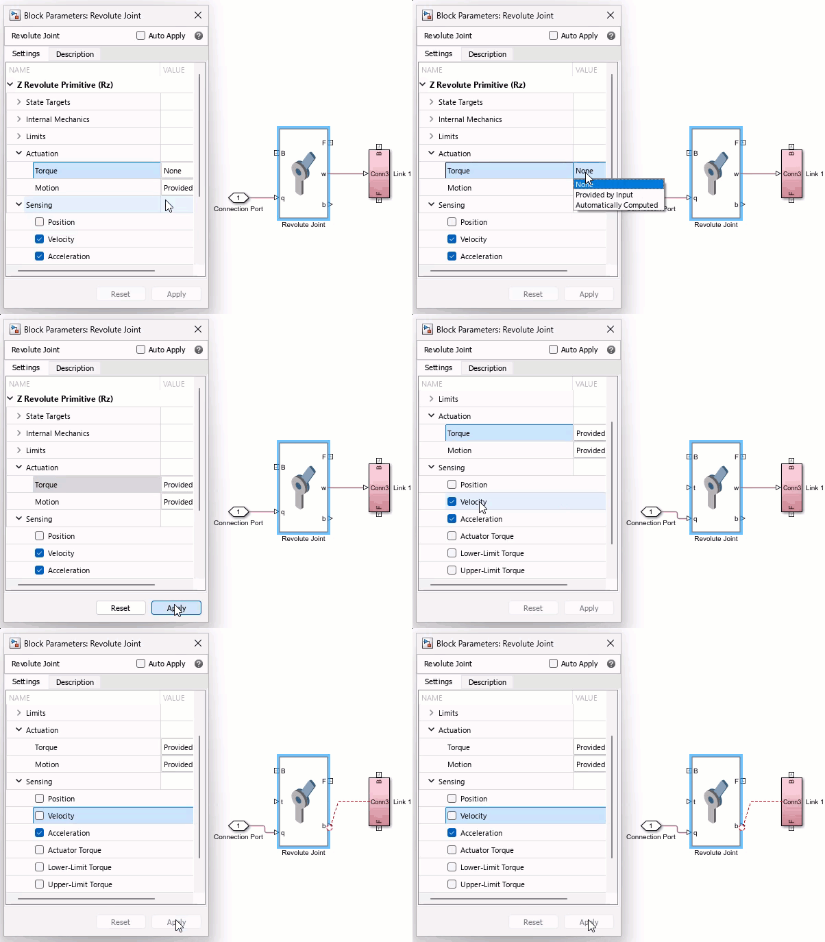
If you set the Torque parameter to Provided by
Input, you expose the physical signal port t and the connection line between the Connection Port block
and port q does not change. In previous releases, this connection line
attached to port t.
If you clear the Velocity parameter check box, you remove port w and the connection line to the Subsystem block disconnects. In previous releases, this connection line attached to port b.
Block Data Sets: Create, manage, and store block parameter data
You can now parameterize Simscape blocks by using a block data set. The partrepo.simscape.BlockDataSet object stores part metadata parameter data that
you can apply to a block. To generate a BlockDataSet object from a block,
use the partrepo.simscape.dataSetFromBlock function.
Simscape uses JSON files to serialize the block data set. You can export block data sets
to a JSON file or retrieve block data sets from an existing JSON file by using the partrepo.exportDataSetsToJSON function or the partrepo.importDataSetsFromJSON function, respectively.
To apply a block data set to a block, use the applyParams
function.
To learn more, see Programmatically Manage Simscape Block Parameter Data.
Simscape Faults Enhancement: Reusable fault definitions
Reuse faults interactively by copying or cutting blocks that have faults assigned and pasting them. Use this feature to add faults to libraries for reuse. To learn more, see Copying Faults.
Functionality being removed or changed
Models that contain Hydraulic library blocks display warnings
Warns
When you run a model that contains Hydraulic library blocks, the model displays a warning. The Hydraulic library will be removed in a future release. To suppress this warning, select Suppress hydraulics deprecation warning in the Hydraulic Fluid block.
Use the hydraulicToIsothermalLiquid function to upgrade your hydraulic models to use isothermal liquid blocks. Blocks in the Isothermal Liquid library provide increased accuracy, usability, and numerical performance.
Use the new subsystemflag argument to minimize the number of blocks
placed into subsystems when you run the hydraulicToIsothermalLiquid function.
Previously, the hydraulicToIsothermalLiquid function placed many
hydraulic blocks into subsystems to reduce the impact of signal rerouting. Now, you can
use the subsystemflag argument to control the subsystems the block
makes. By default, subsystemflag is
"omitsubsystems", and the function only uses subsystems if the
function replaces a single Hydraulic block with multiple Simscape blocks. Even when
subsystemflag is "omitsubsystems", in many
models line rerouting is minimal. If you specify subsystemflag as
"addsubsystems", the function places blocks that impact line
routing into subsystems to fully preserve the Hydraulic model line routing.
Default parameter values of the Thermal Liquid Settings (TL) block have been adjusted
Behavior change
The default parameter values of the Thermal Liquid Settings (TL) block have been adjusted to match the corresponding values in the domain file:
Maximum valid temperature changed from
363.16 Kto373.16 K.Minimum valid pressure changed from
0.05 MPato0.01 MPa.
This change has no compatibility impact. If your model contains a Thermal Liquid Settings (TL) block from a previous release, its parameter values do not change.
Simulation
DAE Solver: Run-time parameter performance improvements
Simulation time may improve when you simulate a model with run-time parameters using a DAE solver. The solver uses improved logic to handle run-time parameters when, in the Solver Configuration block, you select Use local solver.
Scalable Compilation: Skip the baseline compilation
For scalable compilation, the Advisory tool lets you analyze your model for unsupported patterns, provides compilation statistics, and makes recommendations on whether to enable scalable compilation. To do this, the tool compiles the model twice: first, without scalable compilation, to calculate the baseline, and then again with applying scalable compilation.
However, after you have decided to enable scalable compilation, you can still use the Advisory tool to try different ways of restructuring your model into repeated components, to optimize the configuration. In this case, you do not need to calculate a baseline, because you are interested only in the scalable compilation statistics for the current configuration. To save time, you can skip the baseline compilation by using this syntax:
sscScalableAdvisor(modelname,subsyspaths,CompareBaseline=false);
where:
modelnameis the name of the model to analyze, specified as a character vector, string, or a handle to the model. This argument is required.subsyspathsis an optional argument that identifies the repeating subsystems in the model.
For more information, see sscScalableAdvisor.
Scalable Compilation: Enhanced support of nonlinear index reduction
Scalable compilation now supports the derivative replacement method of nonlinear index reduction. Nonlinear index reduction is a global transformation used for solving high-index nonlinear equations. In R2024b, only the projection method was supported. For more information, see the Index reduction method parameter of the Solver Configuration block.
Compilation Speed Enhancement: Declaration function caching
Many Simscape blocks, such as heat exchangers or bipolar transistors, use declaration functions to compute derived parameter values and initialize variables. Previously, these computations were performed every time the model was compiled. Now, the computation results of declaration functions are included in the cached model compilation artifacts. This enhancement speeds up model compilation because the parameter and variable values do not need to be recomputed, unless the underlying block parameters have changed.
If your custom block uses a declaration function for random number generation, caching can lead to unexpected simulation results because the values are reused for subsequent simulation runs and therefore are no longer random. If your model relies on a declaration function generating random parameter or variable values at every simulation run, you can use the new Cache compilation artifacts model configuration parameter to turn off caching.
This restriction applies only if you use functions like rand,
randi, or randn inside a MATLAB declaration function. If you call rand,
randi, or randn directly from Simscape code, for example, use it in a Simscape function or directly in a parameter declaration, caching does not apply.
Improved handling when simulating with local solvers
Local solver enhancements improve simulation time for some models when, in the Solver Configuration block, you select Use local solver and clear Resolve indeterminate equations during runtime. Generated code now has improved performance with a smaller footprint.
Simulation results may differ slightly from previous releases.
Refine output to avoid spikes at zero crossings
Use the new model configuration parameter on the Solver pane, Continuous state refinement method, to refine output and avoid spikes at zero crossings:
Solver interpolation(default) — Use solver interpolation between major steps for zero-crossing detection and state refinement. This behavior is the same as in previous releases.Solver stepping— Use the solver discretization method, effectively taking shorter steps between the major steps and applying the solver discretization formula at refined points. This option has higher computational cost but may produce a solution that better satisfies the equations and avoids spikes at zero crossings.
To enable this parameter, set the Solver parameter to
daessc (DAE solver for Simscape).
Operating Point Enhancements: Display operating point data in table format
You can now use the simscape.op.targetTable function to generate a MATLAB table display of a
Simscape operating point data for visual inspection or programmatic access. To generate an
operating point table, use the
syntax:
opTable = simscape.op.targetTable(op);
simscape.op.targetTable function takes a Simscape operating point,
op, and returns the MATLAB table, opTable.Simscape-to-HDL: Generate fixed-point bitstreams and improved implementation models
When you use Simscape-to-HDL code generation, you can now:
Generate FPGA bitstreams from Simscape models with tunable run-time parameter values when, in the Solver Configuration block, you select Use local solver and set Solver type to
Trapezoidal.Generate improved HDL-optimized models when you use the
sschdl.generateOptimizedModelfunction.
To learn more about R2025a Simscape-to-HDL features, see Release Notes for HDL Coder (HDL Coder).
New examples
Examples introduced in this version include:
Functionality being removed or changed
Improved equation scaling
Behavior change
Enhancements and optimizations for run-time scaling of equations in this release result in better simulation robustness. Certain poorly scaled models where the solver previously failed to find a solution now simulate successfully.
Because of equation scaling optimizations, there may be slight differences in simulation results compared to R2024b.
Simscape Language
Fault Annotations: Model faults in custom components
You can use the Simscape faults interface in custom blocks by adding faults in the
annotations section of the component file. For more
information, see Fault Annotations.
Block Icon Editor: View and edit custom block icons
You can use the Graphical Icon Editor to view and edit block icons for Simscape blocks. To open the editor, select a custom block and, at the MATLAB command prompt, type:
Simulink.IconEditor.open(gcb)
For more information, see Using the Graphical Icon Editor.
Moist Air Domain Definition: Model water droplets suspended in moist air flow
The moist air domain definition has changed to include the addition of droplet tracking. For more information, see Moist Air Domain.
If you have custom Simscape language blocks in the moist air domain, you must update the component code. If your custom block is based on an existing Simscape block, refer to the changes in the Simscape block source code.
The custom moist air blocks now:
Interpolate the specific heat from the
cp_a_TLU,cp_w_TLU,cp_g_TLU, andcp_d_TLUparameters. The domain parameterscp_a_coeff,cp_w_coeff, andcp_g_coeffno longer exist.Modify any specific enthalpy and isentropic relations to include the contribution from water droplets.
Include an additional water droplet mass conservation equation.
Add water droplets to the equations that equate variables for the
port_convectionsubcomponents.
You may need to make additional changes depending on the block. For more information, refer to changes in the Simscape blocks source code.
Functionality being removed or changed
Functions for building and protecting custom libraries have been renamed
Still runs
The functions for building and protecting custom libraries have been renamed.
| Old Name | New Name |
|---|---|
ssc_build | sscbuild |
ssc_mirror | sscmirror |
ssc_protect | sscprotect |
ssc_clean | sscclean |
The old functions, ssc_build,
ssc_mirror, ssc_protect, and
ssc_clean, still run, but will be removed in a future release.
Use the corresponding new function instead. Syntax and arguments of the new functions
are identical to the old ones. To update your code, just remove the underscore ("_")
in function calls.
Foundation Library
Position-Based Mechanical Translational Domain and Block Library: Use position-based modeling framework to model mechanical translational systems
You can use the new position-based mechanical translational domain and the Translational block library to model mechanical translational systems where it is important to know the component positions, for example, valve component assemblies. The Translational block library contains basic building blocks, such as mass, spring, and damper blocks, as well as sources and sensors. The Utilities sublibrary contains the Mechanical Translational Properties (PB) block, which specifies the global parameters for all the blocks in the attached circuit. The Utilities sublibrary also contains the Interface (PB-Translational) block, which allows connections between position-based and non-position-based mechanical translational ports.
For more information, see Modeling Position-Based Mechanical Translational Systems and the block reference pages. Also see Position-Based Translational Domain for information about the new domain definition.
Moist Air Domain: Model water droplets suspended in moist air flow
In applications such as aircraft environment control systems (ECS), the temperature of the bulk moist air can cool quickly enough that the entire volume of air becomes saturated. When this happens, water vapor condenses into liquid water droplets suspended in the moist air flow. Previously, blocks in the Moist Air domain assumed that any condensed water left the moist air network. You can now model water droplets suspended in a moist air flow.
To model water droplets in the moist air flow, select Enable entrained water droplets in the Moist Air Properties (MA) block connected to your moist air network.
Modeling water droplets in moist air allows you to:
Allow condensation to turn into entrained water droplets instead of leaving the moist air flow.
Keep track of entrained water droplets in the domain as they are convected by the moist air flow from one component to another.
Model the re-evaporation of entrained water droplets when the moist air is no longer saturated.
You can now use the Moisture Source (MA) block to directly add water droplets to the system. You can also use the new Moisture Separator (MA) block to remove water droplets from the network. Additionally, these blocks have been updated to be compatible with modeling entrained water droplets:
The Controlled Reservoir (MA) and Reservoir (MA) blocks have been combined into the Reservoir (MA) block.
The Humidity & Trace Gas Sensor (MA) block is now the Moisture & Trace Gas Sensor (MA) block.
In blocks that model fluid volume, such as the chamber, pipe, or mechanical converters, water vapor can condense, condensation can turn into entrained water droplets, and water droplets can evaporate back into the moist air. These blocks also now have initial condition parameters, instead of initial variable targets, that you can use to specify the fluid properties at the start of the simulation.
This change has no compatibility impact when you use these Foundation library blocks in your models. When you open an existing model, the moist air blocks update automatically. However, if you use the Controlled Reservoir (MA) or Humidity & Trace Gas Sensor (MA) blocks in your custom composite components, you must update the composite component code.
Probe Block Enhancement: Use Property Inspector or command-line interface to specify variables to probe
The workflow for selecting which variables to probe has been enhanced and streamlined by introducing the use of Property Inspector. To open the Property Inspector, select a Probe block and press Ctrl+Shift+I or, on the Modeling tab of the model toolstrip, in the Design section, select Property Inspector.
The Property Inspector window contains the name of the block being probed, such as Rotational Electromechanical Converter, and a table of all the block variables that can be probed. Once you select a variable to probe, you can expand it in the table to view the associated port label and unit.
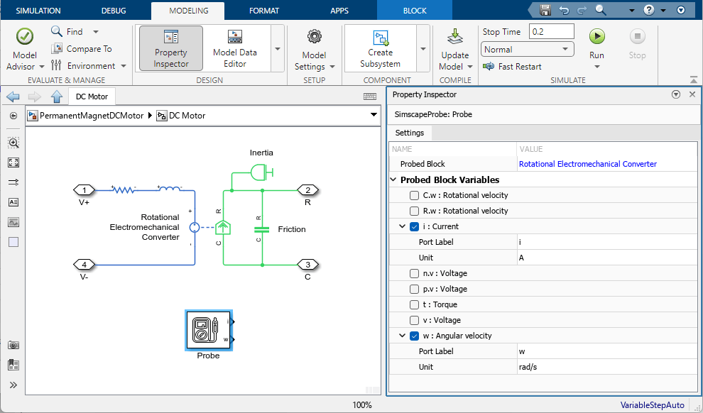
You can also use command-line interface:
simscape.probe.defaultVariableTable(— Construct ablockName)VariableTableobject containing all the variables that can be probed for a specified Simscape block. The function argument is the Simscape block name, specified as a string scalar, character vector, or a handle.simscape.probe.setVariableTable(— Attach an existingprobe,VariableTable)VariableTableto a Probe block. The first argument is the Probe block name, specified as a string scalar, character vector, or a handle, and the second argument is thesimscape.probe.VariableTableobject.simscape.probe.getVariableTable(— View theprobe)VariableTablecurrently attached to a Probe block. The function argument is the Probe block name, specified as a string scalar, character vector, or a handle.
Enhancements to Spectrum Analyzer block
In R2024b, the Spectrum Analyzer block has the following enhancements:
Adaptive RBW: Display spectral data for any number of input samples and adjust RBW accordingly
Previously, spectrum analyzer required a minimum number of samples to update the display for a given RBW value. Starting in R2024b, this limitation is removed. The scope now updates its display for any number of input samples and adjusts the RBW value accordingly.
Window invariant samples per update: Adjust RBW value to always require 1024 samples per spectral update
The spectrum analyzer can now automatically adjust the resolution bandwidth (RBW) such that it always requires 1024 samples per spectral update (Nsamples = 1024) irrespective of the window you choose.
Higher display precision in Spectrum Analyzer UI
You can now increase the display precision to 15 digits using the Display Precision property in the spectrum analyzer settings under Display and Labels. This precision affects all the measurements data and the data the scope displays on its status bar.
To open the spectrum analyzer settings, open the Scope tab of the spectrum analyzer toolstrip, and click Settings.
Preserve Colors is now available in spectrum analyzer toolstrip
The Preserve colors for copy to clipboard property has been renamed to Preserve Colors and is now available in the spectrum analyzer toolstrip under Copy Display.
Maximum number of ACPR offset pairs has increased to 64
Starting in R2024b, the number of ACPR offsets that the spectrum analyzer supports has increased from 12 to 64. You can now set Num Pairs in the Channel Measurements tab to 64.
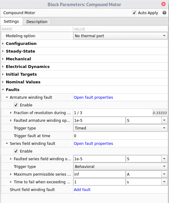
Create faults with default settings
When you add a new fault, the Add fault hyperlink now automatically creates a fault and fault behavior using the default settings. Additionally, you can edit fault properties from the block dialog box.
Functionality being removed or changed
ssc_new has been renamed to
sscnew
Still runs
To create a new model, use sscnew
instead of ssc_new. Syntax and arguments of the two functions are
identical.
ssc_new still runs, but will be removed in a future release.
Use sscnew instead.
Simulation
Selective logging enhancements
When you select a Simscape block variable in the Simscape Variables tab of the Model Data Editor, you automatically enable the block for logging. Clearing all of the variables for a block disables logging on the block.
Additionally, Simscape selective logging now supports rapid accelerator mode and Simulink Compiler.
To learn more about selective logging, see Log Selected Block Variables.
The simscape.instrumentation.enableLogging and
simscape.instrumentation.disableLogging functions will be
removed in a future release and now return a warning. The
simscape.instrumentation.isLoggingEnabled function result now
checks whether the specified Simscape block has one or more block variables
selected.
Disk Caching: Store cached compilation artifacts on disk
Simscape software speeds up compilation of large models by automatically caching compilation artifacts in memory. However, memory caching does not persist between MATLAB sessions. Therefore, when you start a new session, the first compilation of a model takes a longer time.
Now, instead of memory caching, you can store cached compilation artifacts on disk. Disk caching further improves performance by speeding up the first compilation of a model in a given session. Use disk caching to accelerate model development and simulation processes between multiple sessions or multiple collaborators.
To enable disk caching, in the Configuration Parameters dialog box, on the Simscape pane, select the Store cached compilation artifacts on disk check box. For more information, see Disk Caching of Compilation Artifacts.
Simscape-to-HDL Enhancements
When you use Simscape-to-HDL code generation, you can now:
Use fixed-point data type precision for Simscape models that contain nonlinear Simscape networks.
Generate a Simulink state-space equivalent model for an individual Simscape network in your model.
Adjust run-time parameter values for Simscape models that contain multiple Simscape networks.
Automatically replace Simscape PMSM blocks with the equivalent Simulink PMSM block and adjust the run-time parameters.
To learn more about R2024b Simscape-to-HDL features, see Release Notes for HDL Coder (HDL Coder).
Solver Configuration Block: Integrate symbolic trigonometry in time formulation
When you set Equation formulation to Time in
the Solver Configuration block, the solver now performs
symbolic integration and eliminates differential equations with trigonometric functions. The
solver eliminates differential equations of the form a*dot(x) =
b*sin(w*t)+c, where a is a compile-time parameter,
b and c are compile or run-time parameters, and
sin is any linear combination of sine and cosine functions.
Symbolic integration of trigonometric functions eliminates additional differential variables and improves performance.
Scalable compilation limitation removed
Scalable compilation now supports nonlinear index reduction, which is a global transformation used for solving high-index nonlinear equations, if both of these conditions are met:
The model uses the projection method of index reduction. In the Solver Configuration block, set the Index reduction method parameter to
Projection.The model has a single level of hierarchy. That is, the referenced subsystems or components do not include any reference to other subcomponents or subsystem references.
Code generation limitation removed
Code generated from Simscape models now supports encapsulated C++ code generation.
Simscape Language
N-Dimensional Physical Signals and Variables: Support N-D arrays throughout modeling and simulation
Prior to R2024a, Simscape language supported N-D arrays of components and nodes and N-D parameters, as well as 3-D and 4-D lookup tables, but for many aspects of modeling and simulation, array support was limited to two dimensions only. This limitation has now been lifted.
You can now declare variables, inputs, outputs, and intermediates as N-D arrays. The Simscape modeling and simulation tools support these N-D quantities:
Data logging — Simscape Results Explorer indicates N-D data in the legend when plotting. The
simscape.logging.Series.valuesmethod has new options for shaping N-D data. The default behavior is the same as prior to R2024a.Selective logging (introduced in R2024a) — Block instrumentation supports N-D data.
Simulation Data Inspector supports N-D Simscape data and displays it like any other N-D quantity.
Probe block — The block outputs a Simulink signal of the same dimensions as the quantity being probed.
Variable initialization — You can set targets for N-D variables in the block dialogs or Property Inspector. Variable Viewer supports N-D variables and shows whether the targets have been satisfied. For higher-dimensional targets and values, the Variable Viewer cells display only the data dimensions, followed by the word
double. This display is consistent with the Workspace Browser.Operating point —
simscape.Value,simscape.op.Target, andsimscape.op.OperatingPointobjects support N-D quantities.
Variable Scaling Analyzer and Statistics Viewer support N-D quantities but use linear indexing to display the results.
movsum and
cumsum Functions: Calculate moving or cumulative
sums in equations
You can now use these functions in the equations
section:
movsum— Calculate the moving sum.cumsum— Calculate the cumulative sum.
For a complete list of functions supported in the
equations section, see Supported Functions.
Foundation Library
Network Coupler Library Enhancements: Support arrays of electrical nodes
These Network Coupler blocks now support arrays of electrical nodes and three-phase connections:
Network Coupler (Inductor)
Network Coupler (Capacitor)
Network Coupler (Voltage-Current)
Network Coupler (Current-Voltage)
Network Coupler (Voltage-Voltage)
Both the Port 1 Interface and Port 2 Interface
subsystems of these blocks now have a new mask parameter, Electrical node array
size. The default value, 1, corresponds to regular
electrical connections. Entering a different parameter value switches to an array of
electrical nodes. The new Use three-phase electrical connections
check box provides an easy way for you to specify a three-phase electrical port
instead.
When breaking connections between two arrays of electrical nodes, set the Electrical node array size parameter to match the size of the two arrays. Because the top-level subsystem is unmasked, you must set this parameter to the same value for both the Port 1 Interface and Port 2 Interface blocks. Similarly, for three-phase electrical ports, you must select the Use three-phase electrical connections check box for both the Port 1 Interface and Port 2 Interface blocks.
If you look under the mask, the Port 1 Interface and Port 2 Interface subsystems contain custom blocks, such as the Controlled Voltage Source or Current Sensor blocks. These custom blocks are based on the equivalent Foundation library blocks but are modified to support vectorized and three-phase electrical nodes.
Graph Importer Tool: Import datasheet graphs into MATLAB data files for use in block parameterization
You can use the new Graph Importer tool to import graphs from part datasheet PDFs, modify the point data, if needed, and then export selected data as MATLAB data files. You can later use these data files for block parameterization.
To open the tool, at the MATLAB command prompt, enter graphImporter.
Local Restriction (2P) Block Enhancement: Use Bernoulli equation to compute pressure losses
The Local Restriction (2P) block has a new parameter, Pressure loss model:
Bernoulli— The block uses the Bernoulli equation, which assumes uniform density from inlet to outlet. This option is sometimes less accurate than theControl volumemethod, but it is more robust and provides faster simulation.Control volume— The block uses the control volume analysis without assuming uniform density. It models the flow from the inlet to the restriction as a flow contraction and the flow from the restriction to the outlet as a flow expansion. This functionality is the same as prior to R2024a.
Use the Bernoulli option when:
The local restriction is operating in a fully subcooled liquid regime. The fluid is approximately incompressible and the uniform density assumption is appropriate.
The local restriction is used as an expansion valve in a refrigeration cycle. The fluid at the inlet is a subcooled liquid coming out of the condenser, therefore the uniform density assumption is appropriate.
The local restriction is operating in a fully superheated vapor regime, but the flow velocity is low subsonic, which is typically the case in HVAC systems. In this case, the density also does not change much and the uniform density assumption is appropriate.
For all other situations, you can also use the Bernoulli
option to trade accuracy for a faster and more robust simulation.
This change has no compatibility impact. The Bernoulli
option is the default setting for new blocks, but when you open an existing model, the
Local Restriction (2P) blocks in it automatically have
the Pressure loss model parameter set to Control
volume.
Spectrum Analyzer enhancements
The Spectrum Analyzer block has the following enhancements:
To customize the spectrum analyzer status bar, you can now click the Customize status bar icon (
 ) on the right side of the status bar.
The Analyzer tab has been renamed to the Scope tab.
Compact display of simscape.Value and simscape.Unit
objects
When you place simscape.Value and simscape.Unit
objects in table, cell, or structure arrays, or in MATLAB classes, the Command Window now displays the values and units of these
objects explicitly. For example:
y.fieldArray = simscape.Value([1.23, 1.234, 1.23456],'m')y =
struct with fields:
fieldArray: [1.2300 1.2340 1.2346] (m)struct2table(y)
ans =

  table

             fieldArray
    ____________________________

    1.23     1.234    1.2346 (m)
Prior to R2024a, you could see only the member object dimensions and type when displaying the cell, structure, or table array, and needed to display the object members individually to see their values and units.
For row vectors greater than maximum width, empty vectors, and for single line display of matrices and row vectors, you can still see only the member dimensions and type. For example:
y.fieldArray = simscape.Value(zeros(0,3),'m')y =
struct with fields:
fieldArray: [0×3 simscape.Value] (m)This display is consistent with the compact display of other object and data types in the Command Window.
Prior to R2024a, the value and unit in a simscape.Value object were
separated by a colon. Now, the Command Window displays the unit in parentheses after the
value.
simscape.Value Object | Old Display | New Display |
|---|---|---|
T = simscape.Value(10, 'degC') |
T =

10 : degC |
T =

10 (degC) |
V = simscape.Value([1 10 5], 'm') |
V =

     1    10     5

: m |
V =

     1    10     5

(m) |
If you use programmatic data postprocessing that relies on the
simscape.Value object display format, you must update your code.
Default Transparent Background for Simscape Blocks
Prior to R2024a, Simscape blocks had a default white background color. If you changed the color of the canvas, this white background stood out and could clash with the overall color scheme of the canvas. Starting in R2024a, Simscape blocks have a transparent background by default, allowing the canvas color to fill in the background of the block.
In a Simscape block context menu, the Format > Background Color > Automatic option is selected by default, which enables background transparency. If you change the background color to any other color, only closed shapes in the block icon are filled with that color.
The Graphical Icon Editor has new options that allow modifications to transparency of a block background. For more information, see Graphical Icon Editor Overview.
If you open a model created using a previous version of Simulink that contains Simscape blocks on a colored canvas in R2024a, then the backgrounds of all Simscape blocks turn transparent. Additionally, the Format > Background Color > Automatic option is automatically selected in the context menu of these Simscape blocks.
If you save and open such a model created in R2024a in an older version of Simulink, Simscape blocks will acquire a white background.
Constant Aspect Ratio on Block Resize
Starting in R2024a, Simscape blocks preserve the block aspect ratio, by default, on resizing.
For blocks that have line connections from ports to the block icon, such as the NPN Bipolar Transistor block, block resizing is constrained to maintain the aspect ratio. To freely resize such blocks, hold down the Shift key while dragging the block boundary to the new position.
Functionality being removed or changed
Hydraulic library has been removed from Library Browser
Still runs
The Hydraulic library has been removed from the Library Browser. The hydraulic domain definition is still provided with the software, and all the hydraulic blocks in your legacy models continue to work as before. However, these blocks no longer receive full production support and can be removed in a future release.
Use the Isothermal Liquid library and domain to model hydraulic systems where the working fluid temperature remains constant during simulation. For information on upgrading your legacy hydraulic models, see Upgrading Hydraulic Models to Use Isothermal Liquid Blocks.
Numerical improvement for low-flow computation in pipes
Behavior change
To improve accuracy for pressure drop inside the pipe at low-speed flows, the momentum balance computations in the Pipe (G), Pipe (MA), and Pipe (2P) blocks have been changed slightly.
There may be slight differences in simulation results compared to releases prior to R2024a, especially when Mach number is low.
Control runtime regularization independently of fixed-cost simulation
Behavior change
The Resolve indeterminate equations check box in
the Solver Configuration block, which applies runtime regularization to solve statically
indeterminate systems, has been renamed to Resolve indeterminate
equations at runtime and moved to a different section of the dialog box.
Previously, you needed to select the Use fixed-cost runtime
consistency iterations check box to enable it. Now, to enable the Resolve indeterminate equations at runtime check box, you need
to select the Use local solver check box and set
Solver type to either Backward Euler
or Trapezoidal Rule. Unless your model contains lossless
parallel flow paths, such as ideal parallel clutches or switches, you can now clear the
Resolve indeterminate equations at runtime check box
and speed up simulation whenever you use these types of local solver, independently of
whether the simulation is fixed-cost or not.
You can no longer turn off runtime regularization for global solvers.
Simulation
Selective Logging: Log individual block variables
You can now log individual Simscape block variables to the logsout workspace variable.
Simscape logs the variables to a Simulink.SimulationData.Dataset
object, so you can combine block data with other Simulink logged data and view the results in the Simulation Data
Inspector. To learn more, see About Selective Logging and Log Selected Block Variables.
You can also manage selective logging instrumentation programmatically. To learn more, see Log Selected Variables Programmatically.
Some Simscape data logging buttons and menu options have been rearranged on the Simscape Block tab, but their behavior is unchanged from prior releases.
simscape.logging.getSimulationLog Function: Identify the latest
simulation log for a model
Use the new function simscape.logging.getSimulationLog to identify the latest Simscape simulation log for a model. This function is helpful when you work with
several models within a session and have multiple simulation log variables in your
workspace. Provide the model name as an argument, and the function returns the latest
simulation log associated with the model.
Variable Viewer: Identify targets applied by an operating point
If a model is initialized from an operating point, the new Target Source column in the Variable Viewer helps identify the source of variable targets.
For variables that have their target set by the operating point, this column displays
Operating Point. For other variables, targets come either from
block-level initialization or from the underlying component file, and the column remains
empty.
Multithreaded Compilation: Additional performance improvements
Multithreaded compilation has been implemented for additional portions of model compilation. This change further improves compilation performance and applies both to reusable and nonreusable components.
Multithreaded compilation is now always enabled by default, regardless of whether component reuse is on or off. For more information, see How to Enable or Disable Multithreaded Compilation.
Reduced stack size in code generation
Code generation is improved to use fewer local variables. This enhancement results in reduced stack size in the generated C code.
Simscape-to-HDL Enhancements
When using Simscape-to-HDL code generation, you can now modify the run-time parameter values in the generated FPGA bitstream for your Simscape models.
You can also automatically replace the common Simscape switches and converter blocks with
their linearized equivalent from the SimscapeFPGAHIL_lib library. To run
automatic replacement on a model or Simscape network, use the
sschdl.generateOptimizedModel function. You can specify a model or
the Solver Configuration block path for a Simscape network.
For example, to linearize a model stored to the variable input,
enter:
linearizedMdl = sschdl.generateOptimizedModel(input);
linearizedMdl, is the linearized version of
input.To learn more about R2024a Simscape-to-HDL features, see Release Notes for HDL Coder (HDL Coder).
Test harness creation enhancement for Simscape models
If you have a Simulink Test™ license and your component under test contains Simscape blocks, the test harness now displays a help area that links to commonly used blocks for each of the associated Simscape domains. This help area facilitates harness creation for these domains. For more information, see Create a Test Harness (Simulink Test).
New examples
Examples introduced in this version include:
Additionally, the Heat Conduction Through Iron Rod example has been significantly expanded to teach fundamental heat transfer concepts.
Functionality being removed or changed
HDF5 (H5) file format for exporting logged simulation data has been removed
Errors
HDF5 (H5) is a legacy file format for exporting logged simulation data when streaming to disk. The default file format has been changed to MLDATX in R2020b. In R2024a, this functionality has been removed.
Use MLDATX file format for exporting logged simulation data.
Sparkline plots of logged simulation data have been removed
Prior to R2024a, you could display sparkline plots of logged simulation data directly on the model canvas. In R2024a, this functionality has been removed.
Use the Simscape Results Explorer or Simulation Data Inspector to view logged simulation data.
Run-time scaling of algebraic equations
Behavior change
Certain solver optimizations, such as equations scaling, now include run-time parameters. Prior to R2024a, equations were scaled at compile time. This enhancement results in improved solver performance for models with run-time parameters.
There may be slight differences in simulation results, especially for models with run-time parameters. For example, the solver can take a different number of time steps than in R2023b.
Simscape Language
Array-Type Conditional Predicates: Perform element-wise conditional operations on arrays
In previous releases, you could not use array predicates in if
statements. Predicates had to be scalar.
Now you can use the new keyword, .if, to perform element-wise
conditional operations with array-type predicates. For example:
component my_comp
inputs
  pred1 = [1 0 0];
  pred2 = [0 0 1];
end
parameters
    A = [1 2 3];
    B = [4 5 6];
    C = [7 8 9];
end
intermediates
    y = .if pred1, A; .elseif pred2, B; .else C; .end
end
... % Other parameters, variables, equations
end
With these input values, the intermediate y evaluates to
[1 8 6] because:
The first element of
pred1is true, so the first value is the first element of parameterAThe second element of neither
pred1orpred2is true, so the second value is the second element of parameterCThe third element of
pred2is true, so the third value is the third element of parameterB
Functionality being removed or changed
Derived class members cannot have the same names as private base class members
Warns
The ability to declare a derived class member with the same name as a private base class member will be removed in a future release.
In previous releases, these declarations were allowed:
component base
  variables(Access=private)
    x=0;
  end
end

component derived < base
  variables
    x=0;
  end
endStarting in R2023b, declaring a derived class member with the same name as a
private base class member generates a warning. Rename one of the declarations. In the
preceding example, rename one of the variables form x to a
different name.
Foundation Library
Centralized Fault Modeling: Inject faults and configure fault behaviors
The new interface for modeling faults in Simscape blocks separates the system model file or files from those that store fault information. Now, you can systematically add faults to models and run scenarios. You can also safely separate the nominal model behavior from the faulted model behavior to avoid safety tasks interfering with design tasks. To learn more, visit Introduction to Simscape Faults.
You can also use the MATLAB command window to find blocks in your model that support faults, find which faults those blocks support, and add faults to a block or array of blocks using these new functions:
Currently, only blocks in the Simscape Electrical and Simscape Battery™ libraries support the non-intrusive fault interface. If your model from R2023a or before includes modified fault parameters, Simscape automatically adds the non-intrusive faults for you and keeps your fault parameters to ensure the simulation results are unchanged when you upgrade to R2023b.
New Physical Signal Blocks: Add constant bias and perform vector operations on physical signals
The new PS Bias block adds a constant bias to the input physical signal.
Additionally, you can use these new blocks to perform vector operations on physical signals:
PS Concatenate — Concatenates two input vectors or two-dimensional matrices into a single output.
PS Sum of Elements — Calculates the sum of elements of a vector or matrix input physical signal.
PS Dot Product — Calculates the scalar dot product of two vector or matrix physical signals.
PS Vector Norm — Computes the Euclidean norm of a vector or matrix input physical signal.
PS Selector — Lets you select one or more elements from the input vector or two-dimensional matrix.
PS Three-Element Demux — Splits a three-element physical signal vector into three scalar physical signals.
Prior to R2023b, the PS Three-Element Demux block was part of the Simscape Electrical product. It was called the Three Element Demux block and was available only in the Simscape/Electrical/Connectors & References library.
This change has no compatibility impact. The block functionality is unchanged. When you open an existing model containing a Three Element Demux block, it is automatically updated to use the PS Three-Element Demux block from the Foundation library.
Floating Reference Block: Measure voltages in floating network
You can use the new Floating Reference block in the Electrical Elements library to measure voltages of other nodes in a floating network.
Permanent Magnet Block: Represent component that passively generates magnetic field
The new Permanent Magnet block in the Magnetic Elements library represents a component that passively generates a magnetic field by modeling a linear relationship between the flux density, B, and the strength of the external magnetic field, H. The linear relationship is valid only where no magnetization or demagnetization occurs in the magnet. Therefore, the block can operate only in the second quadrant of the B-H curve, where B ≥ 0 and H ≤ 0.
Mach Number Sensor (G) Block: Measure Mach number in the gas domain
The new Mach Number Sensor (G) block in the Gas/Sensors library represents an ideal sensor that lets you measure the Mach number of the gas flow. This block is helpful when you model subsonic compressible flow in the gas domain.
Place the sensor in the flow path you want to measure. The block outputs the Mach number as a unitless value.
Usability Enhancements for Sources: Reduce clutter and improve block diagram layout
Source blocks in the gas, moist air, thermal liquid, and two-phase fluid domains have been streamlined and reconfigured to improve block usability. The high-level changes are:
In each domain, separate Mass Flow Rate Source, Controlled Mass Flow Rate Source, Volumetric Flow Rate Source, and Controlled Volumetric Flow Rate Source blocks have been combined into a single Flow Rate Source block that lets you select between generating constant or time-varying mass flow rate or volumetric flow rate.
In each domain, separate Pressure Source and Controlled Pressure Source blocks have been combined into a single Pressure Source block that lets you select between generating constant or time-varying pressure differential.
Similarly, in the Moisture & Trace Gas Sources library, separate Moisture Source (MA) and Controlled Moisture Source (MA) blocks have been combined into a single Moisture Source (MA) block. Separate Trace Gas Source (MA) and Controlled Trace Gas Source (MA) blocks have been combined into a single Trace Gas Source (MA) block.
These changes help to reduce clutter and improve the block diagram layout.
This change has no compatibility impact when you use these Foundation library blocks in your models. When you open an existing model, the source blocks update automatically. However, if you use these blocks in your custom composite components, you need to update the composite component code.
Network Coupler Library Enhancements: Support arrays of thermal nodes
The Network Coupler (Thermal Mass) block now supports arrays of thermal nodes. If you look under the mask, the Port 1 Interface and Port 2 Interface subsystems contain custom blocks, such as the Controlled Temperature Source or Heat Flow Rate Sensor blocks. These custom blocks are based on the equivalent Foundation library blocks but are modified to support vectorized thermal nodes.
Both the Port 1 Interface and Port 2 Interface
subsystems of the Network Coupler (Thermal Mass) block now
have a new mask parameter, Thermal node array size. The default
value, 1, corresponds to regular thermal connections. However, some
models use arrays of thermal nodes, for example, to connect a battery pack modeled using
Simscape
Battery to a corresponding cooling plate. In this case, there are multiple thermal
nodes in the battery pack that have corresponding thermal nodes on the cooling plate. You
can use the Network Coupler (Thermal Mass) block to separate the two
networks, so that you can use a slower sample time for the thermal part and a faster one
for the electrical part. Using the Network Coupler (Thermal Mass) block in
such a model helps speed up desktop simulation and makes it easier to deploy the model to
real-time hardware.
When breaking connections between two arrays of thermal nodes, set the Thermal node array size parameter to match the size of the two arrays. Because the top-level subsystem is unmasked, you must set this parameter to the same value for both the Port 1 Interface and Port 2 Interface blocks.
Additionally, the default values of the Volume parameter in the Network Coupler (Constant Volume Chamber (IL)) and the Volume and Initial temperature parameters in the Network Coupler (Constant Volume Chamber (TL)) block have been changed to match the default values of the corresponding Foundation library blocks, Constant Volume Chamber (IL) and Constant Volume Chamber (TL).
These changes have no compatibility impact. If you open an existing model containing these blocks, the parameter values and simulation results are the same as in previous releases.
Diode Block Enhancement: Reduce chattering when diode operates near forward voltage
The equations for the Diode block in the Electrical Elements library have been enhanced to reduce zero-crossings when the diode operates near the forward voltage.
Variable Resistor Block Enhancement: Use thermal port to connect resistor to thermal network
The Variable Resistor block in the Electrical Elements library now has an optional thermal port, H. Use this port to connect the resistor to a thermal network. To expose the thermal port, select the Add thermal port check box and specify the thermal mass of the resistor by using the Thermal mass parameter. You can also specify the initial target for the Temperature variable. The block does not model other effects, such as the changes in resistance based on temperature.
Probe Block Enhancement: Select or unselect all variables to probe
To facilitate working with long lists of variables, when you select variables for probing, the context menu now contains an additional check box at the top of the list, just below the Type to Filter field. Toggle this check box to select all or unselect all of the currently listed variables. You can use this check box together with filtering to select or unselect groups of variables.
Spectrum Analyzer supports dBuV units
The Spectrum Analyzer block can now display the spectrum in dBuV
units when you set the type of spectrum to RMS.
Functionality being removed or changed
Moisture & Trace Gas Cap (MA) block has been removed
Starting in R2019b, you do not need to use the Moisture & Trace Gas Cap (MA) block because all Moist Air library blocks with a finite moist air volume have the Moisture and trace gas source parameter, which controls the visibility of port S. The block issued a warning in previous releases. In R2023b, this block has been removed.
To update your legacy models, in each block formerly connected to a
Moisture & Trace Gas Cap (MA) block, set the
Moisture and trace gas source parameter to
None. Then delete the Moisture & Trace
Gas Cap (MA) blocks and unused connection lines.
Consistent reference state for specific enthalpy in moist air domain
Behavior change
Specific enthalpy is a thermodynamic quantity that is measured with respect to a reference state. Sometimes, the specific enthalpies of different gas species can have different reference values. If the upstream and downstream volumes have different mixture composition, flow reversal between these two volumes can result in a nonphysical temperature spike at the node because of upwind calculations and a mismatch in reference temperatures, which in turn can lead to simulation errors.
To ensure consistency in a moist air mixture, the specific enthalpies must have the same reference temperature. Therefore, starting in R2023b, the moist air domain uses a consistent reference temperature of 0 degC. When you enter specific enthalpy vectors in the Moist Air Properties (MA) block, the block internally shifts these vectors to be 0 kJ/kg at 0 degC. The library blocks then use these adjusted values in the internal calculations. The simulation data log also displays the adjusted specific enthalpy values.
The Thermodynamic Properties Sensor (MA) block has a new parameter, Enthalpy reference state, with multiple output options:
As provided in Moist Air Properties (MA) block— The sensor outputs mixture enthalpy based directly on the enthalpy vectors provided in the Moist Air Properties (MA) block, with no adjustments. This option is for informational purposes only because the library blocks now use adjusted values. This option lets you view the same output as in previous releases.0 degC with water as vapor— The sensor outputs mixture enthalpy adjusted to reference state of 0 kJ/kg at 0 degC. These are the values used in the library blocks and shown in the simulation data log.0 degC with water as liquid— The sensor outputs mixture enthalpy adjusted so that liquid water has the reference state of 0 kJ/kg at 0 degC. In this case, enthalpy of water vapor includes the enthalpy of vaporization, or latent heat, at the reference state. These are the values used in the wall condensation calculations.
Because of the automatic shifting, the specific enthalpy values in the simulation
data log can be different than in the previous releases. Use the
Thermodynamic Properties Sensor (MA) block to view
the specific enthalpy values adjusted with respect to different reference states. The
As provided in Moist Air Properties (MA) block option
outputs the same values as in previous releases.
New location for the pm_units.m file
Behavior change
The pm_units.m file contains physical unit names and definitions
registered with the unit Manager. You do not interact with this file directly. Use the
pm_addunit and pm_getunits functions to add new units or get information about the unit
registry. However, you can open this file to see how the physical units are defined in
the product, and also as an example when adding your own units.
In previous releases, this file was located in the folder
matlabroot\toolbox\physmod\common\units\mli\m.
Starting in R2023b, because of the Unit Manager code restructuring, the
pm_units.m file is located in
matlabroot\toolbox\physmod\common\units2\mli\m.
This change has no compatibility impact.
Simulation
Incremental Code Generation: Reduce compilation time by generating code only for the parts of a model that changed
Incremental compilation helps reduce compilation time by reusing compilation artifacts for subsequent compilations in the same session, unless the component was modified between simulation runs. Previously, code generation for these models was not incremental: even if the incremental compilation was enabled, the compiler generated code for the whole model. Now, the compiler generates code only for the parts of the model that have changed between simulation runs.
For more information, see Enable Component Reuse During Compilation.
Multithreaded Compilation: Compile different reusable components on separate threads
Multithreaded compilation helps reduce compilation time by compiling different reusable components on separate threads. Previously, multithreaded compilation of reusable components was not available.
Now, on a multicore machine, if you enable component reuse during compilation, multithreaded compilation is enabled by default. However, if you require single-thread compilation, such as when you are profiling the compilation performance of a model over multiple runs and want to get comparable results, you can disable multithreaded compilation. In the Configuration Parameters dialog box, at the bottom of the Simscape pane, under Advanced Parameters, clear the Enable multithreaded compilation check box.
You can also use the equivalent command-line interface to set the model configuration parameter:
set_param(bdroot,'SimscapeMultithreadedCompilation','off')
Simscape to HDL Workflow Enhancements: Improve usability and results
The Simscape to HDL workflow features these updates:
Validation Mismatches
The Simscape HDL Workflow Advisor now helps you prevent validation mismatches in your HDL implementation models. Validation mismatches may occur when you enable multitasking, because multitasking is not supported for HDL code generation.
To avoid validation mismatches, in the Configuration Parameters dialog box under Tasking and sample time options, clear the Treat each discrete rate as a separate task checkbox.
Updating your model with these configurations may expose rate transitions that Simscape previously handled automatically. You may need to add explicit rate transitions to your system for these cases before you generate HDL code.
Streamlined HDL Code Generation Workflow
The Simscape HDL Workflow Advisor now combines the extraction and discretization steps of the workflow. Previously, Extract equations and Discretize equations were separate steps. Now the step is Extract discrete equations. This change streamlines the workflow and does not impact code generation results.
To learn more, visit Release Notes for HDL Coder (HDL Coder).
Simscape Results Explorer Usability Enhancements
In this release, the Simscape Results Explorer usability enhancements are:
You can now open the Simscape Results Explorer by double-clicking the simulation log workspace variable name.
The Axes Control section of the Simscape Results Explorer toolstrip has been redesigned. Instead of the Limit time axis drop-down, there are now separate fields for setting Start Time and Stop Time, as well as Restore Default Limits and Set to Current Plot Limits buttons.
Example Updates: Open example models from the documentation or command line
As of R2023b, you must use openExample
to open Simscape example models from the command line. You can still access the example models
from the documentation. For instance, to open the Mass-Spring-Damper with Controller example from the
command line,
enter:
openExample('simscape/MassSpringDamperWithControllerExample')| R2023a and before | R2023b |
|---|---|
| ssc_actuator_custom_pneumatic | ActuationCircuitWithCustomPneumaticComponentsExample |
| ssc_aircraft_ecs | AircraftEnvironmentalControlSystemExample |
| ssc_auto_ev | ConfiguringAnEVSimulationForMultirateHILExample |
| ssc_bipolar_nonlinear | NonlinearBipolarTransistorExample |
| ssc_bipolar_smallsignal | SmallSignalBipolarTransistorExample |
| ssc_brayton_cycle | BraytonCycleGasTurbineWithCustomComponentsExample |
| ssc_bridge_rectifier | FullWaveBridgeRectifierExample |
| ssc_building_ventilation | BuildingVentilationExample |
| ssc_cavitation_two_phase_fluid | CavitationInTwoPhaseFluidExample |
| ssc_choked_orifice | ChokedFlowInGasOrificeExample |
| ssc_circuitbreaker | CircuitBreakerExample |
| ssc_dcmotor | PermanentMagnetDCMotorExample |
| ssc_electrochemical_battery | BatteryCellWithCustomElectrochemicalDomainExample |
| ssc_electrolyzer | PEMElectrolysisSystemExample |
| ssc_engine_cooling_system | EngineCoolingSystemExample |
| ssc_fluid_vaporization_in_pipe | FluidVaporizationInPipeExample |
| ssc_fuel_cell | PEMFuelCellSystemExample |
| ssc_house_heating_system | HouseHeatingSystemExample |
| ssc_hydraulic_actuator_analog_control | HydraulicActuatorWithAnalogControlHExample |
| ssc_hydraulic_actuator_analog_control_dashboard | HydraulicActuatorWithAnalogControlWithDashboardHExample |
| ssc_hydraulic_actuator_digital_control | HydraulicActuatorWithDigitalPositionControllerHExample |
| ssc_hydraulic_actuator_HIL | HydraulicActuatorConfiguredForHILTestingHExample |
| ssc_hydraulic_cavitation_cycle | CavitationCycleExample |
| ssc_ideal_hard_stop | MassOnCartUsingAnIdealHardStopExample |
| ssc_il_actuator_analog_control | HydraulicActuatorWithAnalogControlExample |
| ssc_il_actuator_analog_control_dashboard | HydraulicActuatorWithAnalogControlWithDashboardExample |
| ssc_il_actuator_digital_control | HydraulicActuatorWithDigitalPositionControllerExample |
| ssc_il_actuator_HIL | HydraulicActuatorConfiguredForHILTestingExample |
| ssc_il_entrained_air | EntrainedAirEffectsExample |
| ssc_lead_acid_battery | LeadAcidBatteryExample |
| ssc_lead_acid_battery_dashboard | LeadAcidBatteryWithDashboardBlocksExample |
| ssc_linkage_mechanism | LinkageMechanismExample |
| ssc_lithium_battery_arrays | LithiumIonBatteryPackWithFaultUsingArraysExample |
| ssc_lithium_battery_with_fault | LithiumIonBatteryPackWithFaultExample |
| ssc_lithium_cell_1RC | LithiumBatteryCellOneRCBranchEquivalentCircuitExample |
| ssc_lithium_cell_2RC | LithiumBatteryCellTwoRCBranchEquivalentCircuitExample |
| ssc_lithium_pack_thermalRunaway | LithiumPackThermalRunawayExample |
| ssc_mass_spring_damper_control | MassSpringDamperWithControllerExample |
| ssc_mass_spring_damper_sl | MassSpringDamperInSimulinkAndSimscapeExample |
| ssc_mass_spring_damper_sl_dbl | DoubleMassSpringDamperInSimulinkAndSimscapeExample |
| ssc_mechanical_system_translational_friction | MechanicalSystemWithTranslationalFrictionExample |
| ssc_mechanical_system_translational_hardstop | MechanicalSystemWithTranslationalHardStopExample |
| ssc_medical_ventilator | MedicalVentilatorWithLungModelExample |
| ssc_motor_thermal_circuit | MotorThermalCircuitExample |
| ssc_nonlinear_electromechanical_circuit | NonlinearElectromechanicalCircuitWithPartitioningSolverExample |
| ssc_nonlinear_inductor | NonlinearInductorExample |
| ssc_op_rlc_transient_response | OperatingPointRLCTransientResponseExample |
| ssc_opamp_bandlimited | BandLimitedOpAmpExample |
| ssc_opamp_differentiator | OpAmpCircuitDifferentiatorExample |
| ssc_opamp_finitegain | FiniteGainOpAmpExample |
| ssc_opamp_inverting | OpAmpCircuitInvertingAmplifierExample |
| ssc_opamp_noninverting | OpAmpCircuitNoninvertingAmplifierExample |
| ssc_oxygen_concentrator | OxygenConcentratorExample |
| ssc_pendulum | PendulumInCartesianAndPolarCoordinatesExample |
| ssc_pi_collision_calculation | CalculatingPiUsingCollidingMassesExample |
| ssc_pneumatic_actuator | PneumaticActuationCircuitExample |
| ssc_pneumatic_actuator_humidity | PneumaticActuatorWithHumidityExample |
| ssc_pneumatic_motor | PneumaticMotorCircuitExample |
| ssc_probe | CircuitBreakerWithProbeBlockExample |
| ssc_pwm_asynchronous | AsynchronousPWMVoltageSourceExample |
| ssc_pwm_discrete | DiscreteTimePWMVoltageSourceExample |
| ssc_rankine_cycle | RankineCycleSteamTurbineExample |
| ssc_rc_circuit_sl | RCCircuitInSimulinkAndSimscapeExample |
| ssc_rc_circuit_sl_cascade | CascadedRCCircuitInSimulinkAndSimscapeExample |
| ssc_refrigeration | TwoPhaseFluidRefrigerationExample |
| ssc_reusefunctions | SimscapeFunctionsExample |
| ssc_rot_system_stick_slip | MechanicalRotationalSystemWithStickSlipMotionExample |
| ssc_round_rod_heat_conduction | HeatConductionThroughIronRodExample |
| ssc_scattered_lookup | CompressorMapWithScatteredLookupExample |
| ssc_shuntmotor | ShuntMotorExample |
| ssc_simple_mechanical_system | SimpleMechanicalSystemExample |
| ssc_solenoid | SolenoidExample |
| ssc_solenoid_magnetic | SolenoidWithMagneticBlocksExample |
| ssc_stirling_engine | GammaStirlingEngineExample |
| ssc_tl_hydraulic_fluid_warming | HydraulicFluidWarmingDueToLossesExample |
| ssc_tl_oil_pipeline | OptimalPipelineGeometryForHeatedOilTransportationExample |
| ssc_tl_water_hammer | WaterHammerEffectExample |
| ssc_transcritical_refrigeration | TranscriticalRefrigerationCycleExample |
| ssc_transformer | ElectricalTransformerExample |
| ssc_transmission_line | TransmissionLineExample |
| ssc_transport_delay | VariableTransportDelayExample |
| ssc_ultracapacitor | UltracapacitorEnergyStorageWithCustomComponentExample |
| ssc_variant_connector_bounded_region | VariantBoundedRegionInElectricalCircuitExample |
| ssc_variant_connector_leaf_region | VariantLeafRegionInMechanicalSystemExample |
| ssc_variant_connector_vc_mask_workspace | MaskWorkspaceVariableInVariantConnectorBlockExample |
| ssc_variant_connector_with_simscape_bus | VariantConnectorBlockWithSimscapeBusBlockExample |
| ssc_vehicle_hvac | VehicleHVACSystemExample |
New examples
Examples introduced in this version include:
Functionality being removed or changed
Spurious impulses removed from mode chart entry
computations
Behavior change
The entry section is an optional section inside a mode chart that
lets you specify the actions to be performed upon entering a mode. These actions are
event variable updates based on the value of a continuous expression immediately before
entering the mode.
In previous releases, the local solver sometimes erroneously captured impulses in models where there were no actual impulse changes, which resulted in incorrect values for the event variables. The algorithm has been modified so that these spurious impulses are removed.
If your model uses components with mode chart entry
sections, your simulation results may be slightly different than in previous
releases. If you are using a local solver either with fixed-cost mode turned off, or
in fixed-cost mode with impulse iterations, there may be slight differences in the
values of the event variables and some mode changes may occur one step later than
before.
Vector format does not apply to scalars
Behavior change
The Vector format parameter in the PS-Simulink
Converter block lets you specify how to output vector physical
signals. When this parameter was introduced in R2022a, the
inherit option applied to scalar physical signals as
well. Starting in R2023b, this parameter no longer applies to scalar physical signals,
and therefore the output format of a time series of a scalar physical signal is a
Simulink 1-D array.
When this feature was first introduced, in models created prior to R2022a, the
Vector format parameter was automatically set to
1-D array, to preserve backward compatibility.
Therefore, this change primarily affects scalar physical signals in models created
in R2022a, R2022b, and R2023a. If you plot the signals, there is no difference in
the results. However, if you output a scalar physical signal to workspace and the
model has the Vector format parameter set to
inherit, the output format is now different.
Simscape Language
Domain Equations: Use equations in domain files
In previous releases, the equations section was allowed only in a
component file. The purpose of this section is to establish the mathematical relationships
between the variables, parameters, inputs, and outputs of the component, the simulation
time, and the time derivatives of each of these entities.
Now you can also include the equations section in a domain file, to
establish the mathematical relationships between the domain Across variables, parameters,
and intermediates. Domain equations propagate to the nodes of the corresponding domain
type. Like the regular component equations, domain equations are executed throughout the
simulation. You can also specify initial domain equations, similar to the initial
component equations, to be executed during model initialization only.
For more information, see Domain Equations.
Scattered Lookup: Perform linear interpolation on a scattered set of data points
Use the scatteredlookup function in the
equations section to compute an output value by
interpolating the query input value against an unstructured, or scattered, set of data
points. Unlike the tablelookup function, these data
points do not need to form a table grid. You provide the coordinates of a set of input
data points and the function value at each of these data points. Then you provide the
coordinates of a query point or points and the
scatteredlookup function returns the corresponding
interpolated function value by using Delaunay triangulation.
The scatteredlookup function supports
two-dimensional and three-dimensional lookup.
For more information, see scatteredlookup.
Functions for Arrays of Components and Nodes: Use array manipulation and query functions on an object array
Simscape language now allows you to use certain MATLAB functions on arrays of components and nodes to concatenate and reshape these
arrays without using for-loops. You can also query an object array size
and then use that size in a parametric expression in this or another object array.
The supported functions are:
Array manipulation:
repmat,cat,horzcat,vertcat,reshape,transpose. These functions perform manipulations on the input object array and return an object array.Array query:
size,numel,ndims. These functions query the size aspects of an object array and return a result of primitive data type. These functions can be evaluated only at compile time.
For more information, see Using MATLAB Functions with Arrays of Components and Nodes.
Foundation Library
Block Dialog Box Enhancement: Use autocomplete and evaluated values for workspace variables
Simscape blocks now let you use autocomplete when you type in the block parameter fields. The autocomplete options include all the workspace variables in the current session.
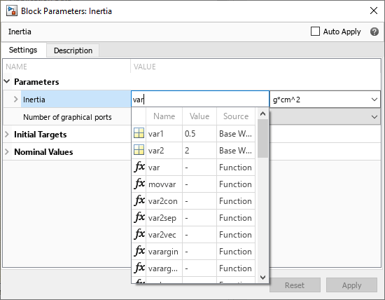
If you set a block parameter to a workspace variable or enter an expression, the block dialog box or Property Inspector evaluates the variable or expression and displays its current value in the parameter field.
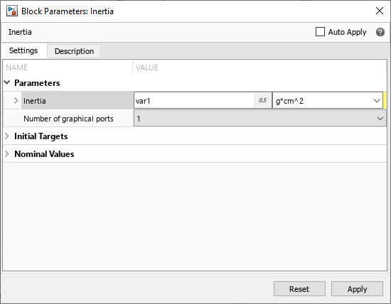
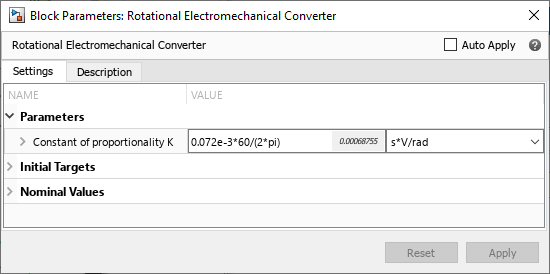
For more information, see View Values of Parameters Set as Variables.
PS Scattered Lookup Table (2D) and PS Scattered Lookup Table (3D) Blocks: Graphically define implicit equations that perform two-dimensional and three-dimensional scattered data lookup
The new PS Scattered Lookup Table (2D) and PS Scattered Lookup Table (3D) blocks in the Physical Signals/Lookup Tables library let you perform Delaunay triangulation on scattered sets of data points:
The PS Scattered Lookup Table (2D) block computes an approximation to some function
f=f(x1,x2)given the coordinates of a set of input data points in a 2D space and function values at each of these data points. The two inputs and the output are physical signals.The PS Scattered Lookup Table (3D) block computes an approximation to some function
f=f(x1,x2,x3)given the coordinates of a set of input data points in a 3D space and function values at each of these data points. The three inputs and the output are physical signals.
For more information, see scatteredlookup.
Probe Enhancement: Select more variables to probe
The Probe block lets you select variables from another block in the model and output them as Simulink signals. In previous releases, when you selected the variables to output, the context menu contained only the variables exposed in the Initial Targets section of the block dialog box. These are the variables that you can use for block-level variable initialization.
Starting in R2023a, the context menu contains all the externally accessible block
variables, regardless of whether they are exposed in the Initial
Targets section of the block dialog box. Externally accessible variables
include: block variables declared with the ExternalAccess attribute
value of either modify or observe, inputs, outputs,
intermediates, modecharts, and domain Across variables at each of the nodes. Essentially,
these are the variables that you can see in the simulation data log.
To facilitate scanning through long lists of variables, especially in composite
components, the display format of variables in the context menu has been reversed from
Name:id to id:Name. For example, instead of
Current:i, the same variable now appears as
i:Current. This view is more consistent with the variable display in
the Variable Viewer, Simscape Results Explorer, and Simulation Data Inspector.
The context menu now also has a filter field at the top. Type in this field to filter the variables displayed in the context menu.
Spectrum Analyzer Block: Use new toolstrip interface to visualize signals
Use the improved Spectrum Analyzer block to visualize the
frequency spectrum of the time-domain signals. The block is more responsive and has a new
toolstrip interface that allows you easy access to spectral analysis, estimation, and
measurement settings. You can configure and display Spectrum Analyzer settings from the
command line with the SpectrumAnalyzerConfiguration object.
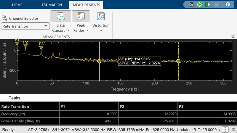
Rotational and Translational Hard Stop Enhancement: Use modeling option based on coefficient of restitution
The Rotational Hard Stop and
Translational Hard Stop blocks have
a new option for the Hard stop model parameter. This option, called
Based on coefficient of restitution, models the hard stop by
using a mode chart that includes free mode, where there is no torque or force transmission
between the slider and the case, and static contact mode, where there is zero speed
difference between the slider and the case. This modeling option improves simulation
performance because static contact mode does not require the block to keep computing hard
stop torque or force when the block is in contact mode.
Variable Thermal Mass Block: Vary thermal mass during simulation
In previous releases, thermal mass stayed constant during simulation. Now, the Thermal Mass block has a new parameter, Mass type:
Constant— The thermal mass is constant during simulation. This option is equivalent to how the block functioned in previous releases.Variable— The thermal mass can vary during simulation. If you select this option, the Mass parameter in the block dialog is replaced by the Minimum mass parameter and a high-priority Mass variable, and the block has two physical signal input ports: Mdot, which specifies the change in the thermal mass, and Tin, which specifies the temperature of incoming mass. The signal value at port Tin has no effect when the thermal mass is constant or decreasing.
Use the Variable option to model systems where the mass
changes but the geometric effects remain negligible, such as a washing machine being
filled, heated, and then emptied with a varying amount of liquid per cycle.
Thermal Liquid Pressure and Flow Rate Sources That Perform No Thermodynamic Work: Configure flow conditions without affecting temperature
All blocks in the Thermal Liquid > Sources library have a new Power added parameter that lets you select whether the source performs work on the fluid flow:
Isentropic power— The source performs isentropic work on the fluid to maintain the specified pressure differential, mass flow rate, or volumetric flow rate depending on the source type. This is the default option, which is equivalent to the block behavior in previous releases. Use this option to represent an idealized pump or compressor and account for the energy input and output, especially in closed-loop systems.None— The source performs no work on the flow, neither adding nor removing power, regardless of the pressure differential or flow rate produced by the source. Use this option to set up the desired flow condition upstream of the system, without affecting the temperature of the flow.
Wet-Bulb Temperature Data: Use wet-bulb temperature to specify and measure humidity in the moist air domain
Wet-bulb temperature is a method of measuring humidity that involves wrapping a wet cloth around a thermometer, so that you can measure the temperature including energy loss due to evaporation. Traditional psychrometers output data in the form of wet-bulb temperature.
These blocks in the Moist Air library now have an option to specify and measure humidity by using the wet-bulb temperature:
Usability Enhancements for Sensors and Sources: Reduce clutter and improve block diagram layout
Sensor blocks in several domains have been streamlined and reconfigured to improve block usability. The high-level changes are:
In the gas, moist air, thermal liquid, and two-phase fluid domains, separate Mass & Energy Flow Rate Sensor blocks and Volumetric Flow Rate Sensor blocks have been combined into a single Flow Rate Sensor block that lets you measure mass flow rate, energy flow rate, and volumetric flow rate.
Sensor blocks with multiple output ports in the gas, moist air, thermal, thermal liquid, and two-phase fluid domains now have conditional port visibility on the block icon. You can use the block parameters to expose only the ports that you need for measurements in a particular model.
Pressure & Temperature Sensor blocks in the gas, moist air, and thermal liquid domains, as well as the Pressure & Internal Energy Sensor (2P) block and the Temperature Sensor block, now contain an implicit reference node, which means that you need only one port to make absolute measurements of pressure, temperature, or internal energy. Expose the second port only if you need to measure the difference in pressure, temperature, or internal energy between two nodes in the model.
These changes help to reduce clutter and improve the block diagram layout.
Additionally, changes to particular blocks include:
In the gas domain, you now have an option to calculate the volumetric flow rate by using density at standard pressure and temperature, rather than at the actual working conditions of the system. The Volumetric Flow Rate Source (G), Controlled Volumetric Flow Rate Source (G), and Flow Rate Sensor (G) blocks have additional parameters that let you switch between actual and standard conditions, and to specify the standard pressure and temperature for calculating the volumetric flow. In previous releases, this functionality was available only in the moist air domain.
The Pressure & Internal Energy Sensor (2P) block has been renamed to Pressure, Temperature & Internal Energy Sensor (2P) because it now also outputs temperature.
The Thermodynamic Properties Sensor (2P) block now also outputs density.
This change has no compatibility impact when you use these Foundation library blocks in your models. When you open an existing model, the source or sensor blocks within it update automatically. However, if you use these sensor blocks in your custom composite components, you need to update the composite component code.
How you update the code depends on the sensor block. For Mass & Energy
Flow Rate Sensor blocks and Volumetric Flow Rate Sensor blocks
in each domain, the source file name has changed to flow_sensor. For
sensors where conditional port visibility has been implemented, add the implicit
reference node and expose additional ports to match the default block behavior in
previous releases. For example, if you declared the Pressure &
Temperature Sensor (TL) block
as
components (ExternalAccess = observe)
    sensorBlock = foundation.thermal_liquid.sensors.pressure_temperature_sensor;
end
components (ExternalAccess = observe)
    sensorBlock = foundation.thermal_liquid.sensors.pressure_temperature_sensor
                  (reference = foundation.enum.MeasurementReference.difference,temperature = true);
end
| Sensor Block to Update | Old Syntax | New Syntax |
|---|---|---|
| Mass & Energy Flow Rate Sensor | sensor =
foundation.gas.sensors.mass_flow_energy_flow_sensor; | sensor = foundation.gas.sensors.flow_sensor; |
| Volumetric Flow Rate Sensor | sensor =
foundation.gas.sensors.volumetric_flow_sensor; | sensor =
foundation.gas.sensors.flow_sensor(volumetric_flow_measure=true); |
| Pressure & Temperature Sensor | sensor =
foundation.gas.sensors.pressure_temperature_sensor; | sensor =
foundation.gas.sensors.pressure_temperature_sensor(reference=foundation.enum.MeasurementReference.difference,
temperature=true); |
| Thermodynamic Properties Sensor | sensor =
foundation.gas.sensors.thermodynamic_sensor; | sensor =
foundation.gas.sensors.thermodynamic_sensor(enthalpy=true,
specific_heat=true, entropy=true); |
Fluid Properties: Simulate beyond range of fluid property tables
In a fluid domain, parameters set the acceptable ranges of fluid properties, such as pressure and temperature. Domain parameters usually specify these ranges either in tabular form, or as minimum and maximum acceptable values. In previous releases, if a variable corresponding to a fluid property went outside the acceptable range during simulation, the simulation stopped with an error.
Starting in R2023a, you can make this error optional. The blocks that define fluid properties for each domain have a new parameter that lets you specify what happens if the fluid properties in the circuit attached to this block go out of range during simulation:
error— Simulation stops with an error. This option is the default setting and preserves the same behavior as in previous releases.warning— Simulation continues but displays a warning that the variable is out of range.none— Simulation continues with no warning.
The parameter name in the fluid properties block varies, depending on the variables in the domain, but the options are the same.
| Domain | Block Name | Parameter Name |
|---|---|---|
| Isothermal liquid | Isothermal Liquid Properties (IL) | Pressure outside valid range |
| Thermal liquid | Thermal Liquid Settings (TL) | Pressure and temperature outside valid range |
| Two-phase fluid | Two-Phase Fluid Properties (2P) | Pressure and specific internal energy outside valid range |
| Gas | Gas Properties (G) | Pressure and temperature outside valid range |
| Moist air | Moist Air Properties (MA) | Pressure and temperature outside valid range |
Note
These parameters apply only to situations when values get out of range during simulation. If you enter out-of-range values in a block dialog box, you get a compilation error regardless of the parameter setting.
Additionally, in the Isothermal Liquid Properties (IL) block, the default value of the Minimum valid pressure parameter has been changed from 0.1 Pa to a more realistic value of 1 Pa.
Port Domain Type Propagation: Speed up editing complex models
When you add connection lines in a block diagram, port domain type propagation computes the port domain type of all linked connection ports in a model. For example, if you add a line between a connection port of a subsystem and a Capacitator block, the Simulink editor resolves this line as an electrical connection. In complex models, where port domain type propagation might take longer to complete, the Simulink editor is locked for editing. Starting in R2023a, a Pause button on the status bar allows you to suspend the ongoing propagation and unlock the editor.
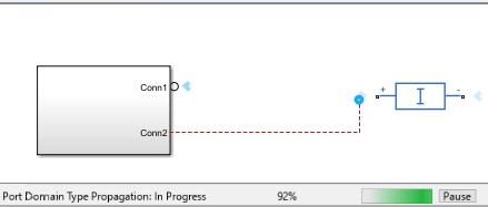
Clicking Pause causes the following behavior:
Port domain type propagation is terminated, and resolved ports hold the correct port domain type and direction. Some percentage of ports might have an unresolved port domain type or direction. If you click Update Model from the Modeling tab or simulate the model at this time, propagation continues for the unresolved ports.
The editor is unlocked for use.
If you continue building your model, any subsequent complex propagation is terminated and is accompanied by a message indicating incomplete propagation.
A Resume button appears on the status bar.
Clicking Resume causes the following behavior:
Port domain types are computed for all ports affected since the last pause operation, including any complex propagation initiated after clicking Pause.
The Resume button is removed from the status bar.
Functionality being removed or changed
Hydraulic library will be removed
Still runs
Hydraulic library will be removed in a future release.
Use the Isothermal Liquid library and domain to model hydraulic systems where the working fluid temperature remains constant during simulation. Blocks in the Isothermal Liquid library provide increased accuracy, usability, and numerical performance. For more information, see Upgrading Hydraulic Models to Use Isothermal Liquid Blocks.
Simulation
Incremental Compilation: Reduce compilation time by recompiling only those parts of a model that have changed
Incremental compilation is an extension of the scalable compilation functionality. Scalable compilation lets you mark subsystems or blocks as reusable, and then reuses compilation artifacts for multiple repeated instances of a component in the same model. Incremental compilation reuses compilation artifacts of reusable components for subsequent compilations within the same MATLAB session, unless the component has been modified between simulation runs.
When you enable component reuse:
During the first compilation, the solver compiles one instance of each reusable component and then reuses these compilation artifacts for repeated instances in the model. This functionality is the same as in previous releases.
During subsequent compilations, the compilation time is further reduced because if a reusable component is unchanged, the solver does not recompile it. This optimization applies to all the reusable blocks and subsystems in the model, independent of whether there are multiple instances or just a single instance.
For more information, see Enable Component Reuse During Compilation.
The mechanism for marking subsystems or blocks as reusable has been consolidated and simplified. In previous releases, there were separate commands for marking subsystems and blocks as reusable and the command for subsystems applied only to referenced and linked subsystems. Now you can designate any subsystem or block as reusable:
simscape.reuse.setConfig(blockPath,'on')
where blockPath is the path to the block or subsystem from the root of
the model.
To disable compilation reuse for a block or subsystem within a model, enter:
simscape.reuse.setConfig(blockPath,'off')
To query the reuse setting for a block or subsystem, enter:
setting = simscape.reuse.getConfig(blockPath)
The command-line interface for setting and getting the component reuse status has been consolidated and simplified. If you have scripts that use the old commands for setting and getting the block or subsystem status for scalable compilation, update them with the new command names and settings:
| Instead of | Use |
|---|---|
simscape.scalable.setSubsystemConfig(blockPath,'auto')
| simscape.reuse.setConfig(blockPath,'on') |
simscape.scalable.setSubsystemConfig(blockPath,'off')
| simscape.reuse.setConfig(blockPath,'off') |
simscape.scalable.setBlockConfig(blockPath,'on')
| simscape.reuse.setConfig(blockPath,'on') |
simscape.scalable.setBlockConfig(blockPath,'off')
| simscape.reuse.setConfig(blockPath,'off') |
simscape.scalable.getSubsystemConfig(blockPath)
| simscape.reuse.getConfig(blockPath) |
simscape.scalable.getBlockConfig(blockPath)
| simscape.reuse.getConfig(blockPath) |
Statistics Viewer Updates: Analyze simulation performance with the improved Statistics Viewer tool
The Statistics Viewer tool features an updated layout to enhance your analysis of model simulation statistics. To view model statistics, in the model window, on the Debug tab, click Simscape > Simscape Statistics. Using the tool, you can
View model statistics including information about the variables and zero-crossings
View statistics about the compilation process
Compare different models or model configurations
Now, when you select a block in the Statistics Viewer tool, you can highlight the block on the model canvas. The View Source button is available when you select a block that experiences a zero-crossing. The button takes you to the relevant equation in the source code.
To learn more, visit View Model Statistics.
Simscape to HDL Compatibility Enhancements: Use Trapezoidal
Rule and real modes
You can now deploy HDL code from models with:
Solver type set to
Trapezoidal Rule.Operators
floor,ceil,round, andmodwithout casting them asint32oruint32.Real-valued discrete variables. This update enables support for the Stepper Motor Driver (Simscape Electrical) block.
To learn more, visit Release Notes for HDL Coder (HDL Coder).
Improved Initialization Diagnostics: Avoid unexpected results when using
OperatingPoint objects
Simscape now features improved handling for OperatingPoint object
initialization. To learn more, visit Using Operating Point Data for Model Initialization.
You may generate different results from previous releases when initializing models
with OperatingPoint objects.
New examples
Examples introduced in this version include:
Simscape Language
Array of Nodes: Define conserving ports as resizable arrays of elements
You can now use arrays and for-loop constructs when declaring
component nodes. Follow these rules:
Arrays, which previously applied only to the
componentsmember class, now also apply to thenodesmember class.Array members must all belong to the same domain.
The array size can be a parameter with the
ExternalAccessattribute set tomodify, which means that the block users can modify this value.Use
for-loops to declare arrays of nodes and to connect members of the array to each other. You can also index into an array of nodes to specify textual connections between elements.Use nested
for-loops to create multidimensional arrays of nodes.
An array of nodes (AON) is represented as a single port on the block icon. If you have two or more AON ports of the same domain type and identical size, you can establish element-wise connections between these arrays by drawing connection lines between the ports. When using AON ports:
Like with scalar ports, error checking for the domain type is performed at edit time. You cannot connect ports of different domain types.
Error checking for the array size is performed at compile time. This means that, although you can graphically connect AON ports of different sizes, this connection generates an error when you compile the model or update the block diagram.
Implicit scalar expansion is not supported. Connecting a scalar port to an AON port also generates a compile-time error.
For more information, see Arrays of Nodes.
Simscape Language Preferences Panel in MATLAB Online: Change default colors and set other preferences for the Simscape language editor
In MATLAB Online™, you can change the colors and other settings used by the Simscape language editor.
To access these settings, on the Home tab, in the Environment section, click Preferences. Select MATLAB > Editor/Debugger > Other Languages > Simscape to open the Simscape language preferences panel.
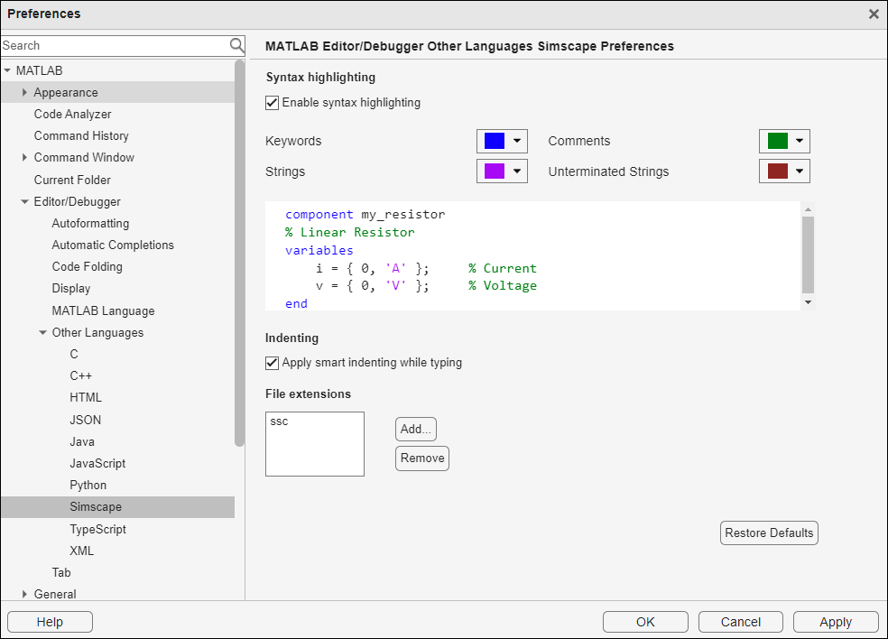
If you change the color for Keywords, Comments, Strings, or Unterminated Strings, the code sample inside the panel reflects your changes. You can also change other settings, such as enable or disable syntax highlighting or smart indenting. When you click Apply, the Editor window reflects these changes.
The Restore Defaults button restores the default Simscape language editor settings.
Foundation Library
Limited PS Integrator: Specify saturation bounds for PS Integrator block
The PS Integrator block can now function as a limited integrator, holding its output within the specified saturation bounds:
When the integral is less than or equal to the lower saturation limit, the block holds the output at the lower saturation limit.
When the integral is between the lower saturation limit and the upper saturation limit, the output is the integral.
When the integral is greater than or equal to the upper saturation limit, the block holds the output at the upper saturation limit.
Use the Limit output parameter to specify whether to limit the output at the lower bound, upper bound, or both. The Limit output source parameter provides two ways of specifying the upper and lower bounds:
Internal— Define the saturation bounds using the Upper limit and Lower limit parameters.External— Define the saturation bounds using the external physical signals at ports U and L.
PS Transfer Function Block Enhancement: Reset block output at events
The PS Transfer
Function block is now resettable at events. You can specify that the
block output resets to the initial output when the physical signal at port
R triggers a reset. The initial output source can now be either a
physical signal or a block parameter. If you set the Initial output
source parameter to External, the physical signal
at port Y0 supplies the initial output value, which is also the
output value after reset.
In the default configuration, with External reset parameter set
to None and Initial output source set to
Internal, the block functions as in previous releases.
Enhancements to Translational and Rotational Motion Sensors: Measure acceleration and parametrically control the visibility of output ports
The Ideal Translational Motion Sensor and Ideal Rotational Motion Sensor blocks have these enhancements:
An additional physical signal output port that lets you measure acceleration.
Additional parameters that control the visibility of physical signal output ports. Use these parameters to expose only the ports that are actually used for measurement in each particular instance. This enhancement helps improve the block diagram readability. Also, because exposing the acceleration measurement port involves additional computations, this port is hidden by default. Do not expose it unless you need to measure acceleration.
In previous releases, the blocks measured only the relative velocity and position of port R with respect to port C. Now, the new Measurement reference parameter lets you disable port C and measure with respect to ground (internal reference node).
Conditional Port Visibility for Two-Phase Fluid Blocks: Expose additional ports in block variants
The source code for the Two-Phase Fluid library blocks has been updated to take advantage of the conditional port visibility and make this library consistent with other fluid block libraries. As a result, the block library has been streamlined by combining similar blocks that differed primarily by the number of ports:
The Constant Volume Chamber (2P) block can now have between one and four ports. The four-port option is new. If a chamber has four ports, you can use it as a junction in a cross connection. Separate two-port and three-port blocks are no longer available. This change has no compatibility impact. All two-port and three-port chamber blocks in existing models are automatically replaced by a Constant Volume Chamber (2P) block with the appropriate number of conserving ports.
The Local Restriction (2P) block can now have an optional input physical signal port that models the variable restriction of flow area. Variable Local Restriction (2P) block is no longer available. This change has no compatibility impact. All Variable Local Restriction (2P) blocks in existing models are automatically replaced by Local Restriction (2P) blocks with an exposed control port.
Pipe (MA) Block Enhancement: Model effect of condensation on wall surface
The Pipe
(MA) block has a new parameter, Condensation on wall
surface, that lets you model the effect of wall condensation on a cold pipe
surface in contact with a moist air volume. Use this parameter when modeling HVAC systems
that contain pipes and ducts. If these pipes and ducts are not well insulated, their
surface could get cold, and condensation on wall surface occurs. When you set
Condensation on wall surface to On, the
convective heat transfer equation accounts for both sensible and latent heat, and the
block also calculates the rate of water vapor condensation on the surface.
Thermal Library Enhancements: Expand heat transfer modeling capabilities and improve diagram layout
Several enhancements in the Thermal library provide additional options for modeling thermal effects within a Simscape network. These enhancements include:
Thermal conductivity in the Conductive Heat Transfer block can be either constant, which you specify by the Thermal conductivity parameter, or variable. You can specify variable thermal conductivity either as a physical signal at port K or as a lookup table based on temperature.
Additionally, you can set Wall geometry to
PlanarorCylindrical.Planarrefers to a flat, rectangular wall.Cylindricalrefers to a round pipe wall.In the default configuration, with Conductivity type parameter set to
Constantand Wall geometry set toPlanar, the block functions as in previous releases.Heat transfer coefficient in the Convective Heat Transfer block can be either constant, which you specify by the Heat transfer coefficient parameter, or variable, which you specify as a physical signal at port K.
In the default configuration, with Convection type parameter set to
Constant, the block functions as in previous releases.The Thermal Mass block can have one or two ports. In some applications, it is customary to display mass or inertia in series with other components in the block diagram layout. To support this use case, you can now display a second port on the block icon. The two-port variant is purely graphical: the two ports have the same temperature, so the block functions exactly the same whether it has one or two ports.
erf and erfc function support for
simscape.Value objects
You can now use erf and erfc when working with simscape.Value objects.
For a complete list of supported functions, see Core MATLAB Functions Supporting simscape.Value Arrays.
Energy and charge units added to unit registry
Additional units in the default Unit Manager registry in this release include:
New energy and charge units based on watt-hour and ampere-hour:
Ah,mAh,kAh,MAh,Wh,mWh,kWh,MWh.Popular multipliers for other units currently in the registry, such as
MV,MA,GW,mOhm,uJ, andmJ.
For a complete list of units in the Unit Manager registry, see Unit Definitions.
Simulation
State-Based Consistency Tolerance: Fine-tune the nonlinear solver tolerances used for computing initial conditions and transient initialization
In previous releases, the Consistency tolerance parameter of the Solver Configuration block had a numeric value, and the block used a nonlinear solver based on the equation residual tolerance to initialize the model. The default parameter value was applicable to most cases. However, the residual-based computation did not provide a clear way to adjust the parameter value and improve the model initialization.
Now, the block uses state-based absolute and relative consistency tolerances, multiplied by a scaling factor, to compute the initial conditions and for transient initialization. The Consistency tolerance parameter of the Solver Configuration block provides a choice:
Model AbsTol and RelTol— Use the model tolerance settings, specified as Absolute tolerance and Relative tolerance parameters on the Solver pane of the Configuration Parameters dialog box.Local tolerance settings— Replace the model tolerance settings with local values. When you select this option, the Absolute tolerance and Relative tolerance parameters appear in the Solver Configuration block dialog box.
Independent of whether you use the model tolerances or the local tolerance settings, the new Tolerance factor parameter provides a scaling factor for these values. The resulting value determines how accurately the algebraic constraints are to be satisfied at the beginning of simulation and after every discrete event, such as a discontinuity resulting from a valve opening or a hard stop. Decrease the parameter value to obtain a more reliable time simulation. Increase the parameter value if solving for initial conditions failed to converge, or to reduce the computation time.
The new state-based method provides better robustness and efficiency, especially if used in conjunction with scaling the model by nominal values.
If you open an existing model where the Consistency tolerance parameter has a numeric value, the model continues to use the same residual-based computation method that it used in previous releases and your simulation results do not change.
To upgrade your existing models to use the new state-based method, use the Check Simscape use of state-based consistency tolerances check in the Upgrade Advisor.
Steady-State Enhancement: Consider mode charts and events for steady-state solution
When you enable steady-state initialization, the solver now selects the steady-state solution that is consistent with the mode charts and event variables present in the model. For more information, see Finding an Initial Steady State.
In previous releases, the solver held mode charts and events in their initial states and found a steady-state solution. The solver then updated mode charts and event variables as a subsequent step. Because the steady-state solution is now consistent with the modes and events, the result can be different than in previous releases.
Multithread Function Evaluation: Speed up fixed-cost simulations that use Backward Euler local solver
If your model uses the Backward Euler local solver, computing Newton iterations is
time-consuming, which may present an issue for fixed-cost simulations. You can now use
multithread function evaluation to speed up simulation on a multicore machine. The new
Maximum threads for function evaluation parameter in the
Solver Configuration block lets you specify the desired
number of threads. The solver reduces the number you specify to the nearest power of 2.
For example, if you specify 5 as the parameter value, the solver uses 4
threads. The default, 1, corresponds to single-thread function
evaluation and is equivalent to the algorithm used in previous releases.
This parameter is available only if you select the Use local
solver check box, set the Local solver parameter to
Backward
            Euler
, and select the Use fixed-cost
runtime consistency iterations check box.
Additionally, to use multithread function evaluation, you must clear the Resolve indeterminate equations check box. This check box is also new in this release. For details, see the Solver Configuration block reference page.
Other unsupported simulation modes for multithread function evaluation include frequency-and-time simulation, delay, scalable compilation, accelerator mode, and rapid accelerator mode. When using multithread function evaluation, you can generate code using Simulink Real-Time™, but other types of code generation are not supported.
Statistics Viewer Enhancement: Provide a more complete reporting of constraint statistics
Typically, the presence of constraints indicates a high-index problem that requires applying index reduction techniques to simplify the system, in order for it to be solved. In previous releases, the Statistics Viewer, under Number of dynamic variable constraints, reported only the number of constraint equations detected during run-time index reduction.
This statistic has been renamed to Number of constraints. This statistic now reports the total number of primary constraint equations in the model, which are the equations the index reduction algorithm handles at compile-time or at run-time. If Number of constraints is greater than zero, the Sources section lists the differential variables involved in each constraint.
Simscape to HDL Compatibility Enhancements: Use averaged switching, input filtering,
unit conversions, tablelookup, and mode charts in Simscape models
If you have an HDL Coder™ license, you can take advantage of more Simscape features when generating FPGA code. When you set Solver
type to Partitioning, you can generate HDL code
from models that contain:
Converter blocks with the Switching device parameter set to
Averaged switch. For more information, see Release Notes for Simscape Electrical (Simscape Electrical).The
tablelookupfunction in the connection functions. You must useinterpolation = linearandextrapolation = linear. The tables must have no more than four dimensions. To learn more about connection functions and systems of equations in the partitioning solver, visit Understanding How the Partitioning Solver Works.Integer-valued events and mode charts.
When you set Solver type to Backward
Euler, you can generate HDL code from models that contain
Simulink-PS Converter blocks with the Input
filtering order parameter set to either First-order
filtering or Second-order filtering.
For both solver types, you can generate HDL code from models that contain PS-Simulink Converter blocks with Output signal unit set to any unit.
For more information, see Release Notes for HDL Coder (HDL Coder).
Functionality being removed or changed
exp function limiting to avoid nonfinite values
Behavior change
If a block uses the exp function in its equations, a very large
value inside that function can cause the exponential to become infinite and thus
introduce Inf or NaN values at initialization time or during simulation.
Starting in R2022b, exponential limiting has been introduced to avoid generating
nonfinite values during initialization and simulation. However, exponential limiting is
not performed when exp is used as an argument inside functions such
as isinf, isnan, or isfinite.
In these cases, the exp function can assume nonfinite values to
ensure the correct predicate evaluation.
This change improves simulation robustness for most models. However, some models can now issue a warning during simulation about the limiting of the exponential.
Change to symbolic integration algorithm
Behavior change
In previous releases, if you simulated a frequency-and-time model that involved only differential variables that were dependent on each other, nonzero initial conditions of such variables were ignored during symbolic integration. In other words, all such variables were assumed to have an initial condition of 0.
Starting in R2022b, the symbolic integration algorithm has been enhanced to account for the initial conditions in this case.
As a result of this change, some models can now initialize differently than in previous releases.
Simscape Language
Scalable Compilation for Textual Components: Reduce compilation time for models containing component arrays
Scalable compilation for models containing a large number of repeated components was
introduced in R2021b. For more information, see Scalable Compilation. In the previous release, the
reusable components had to be included in the model as either referenced subsystems or
linked subsystems. This functionality has now been extended to include textual components.
A new attribute, CompileReuse, lets you specify whether the components
are reusable or not. This attribute is available for components only. If set to
true, the compilation artifacts for these components are reusable.
The default is false.
For example, if you model repeated components by using component arrays, you can use
the CompileReuse attribute to specify which component arrays are
reusable:
component battery_pack
...
for i =1:Ncells
    components(ExternalAccess=none,CompileReuse=true)
        battery_cell(i) = BatteryPack.battery_cell(cell_mass=cell_mass);
    end
    ...
end
...
for i=1:Ncells-1
    components(ExternalAccess=none)
        conduction(i) = foundation.thermal.elements.conduction(area={1e-3,'m^2'},...
            th_cond={200,'W/(m*K)'});
    end
    ...
end
...
If scalable compilation is enabled for a model containing this battery pack component,
then the members of the first component array, battery_cell, are
reusable. Members of the second array, conduction, are not designated
as reusable because the conduction element in the Foundation library is not complex enough
to benefit from scalable compilation.
LoggingUnit Annotation: Specify the preferred display unit for
intermediates, variables, inputs, and outputs
A new annotation option, LoggingUnit, lets you specify a preferred
data logging unit for component members, such as intermediates, variables, inputs, and
outputs. If specified, the same unit is also used for other display purposes, such as in
the Variable Viewer or in the operating point.
The specified logging unit must be commensurate with the intrinsic unit of the component member, such as the declared unit of a variable, typed input, or typed output. For intermediates and untyped inputs and outputs, the intrinsic unit is computed by the compiler. For example:
component mycomp

parameters
  p1 = {10,'lb'};
  p2 = {5, 'ft'};
end

intermediates
  i = p1*p2;
end

annotations
  i : LoggingUnit = 'J'
end

...Foundation Library
Standalone Property Inspector for Simscape Blocks: Unified look and feel of the block user interface
In previous releases, double-clicking a Simscape block opened the block dialog box, where you viewed the block description and modified its parameters. Alternatively, you could view and modify the block properties in the Property Inspector pane in the model window.
Starting in R2022a, when you double-click a Simscape block, the Property Inspector opens in a standalone window. This window has the same content and appearance as the Property Inspector pane in the model window.
To view and modify the block parameter values and initialization targets for the block variables, double-click the block, click the Settings tab, and modify the values of the parameters, variable priorities, and targets.
By default, changing a value in the Property Inspector immediately applies the new
value. To remove a series of changes, use the Undo  button and Redo
  button in the upper-right corner of the model window.
To manually apply parameter changes, clear the Auto Apply check box in the upper-right corner of the Property Inspector to enable the Reset and Apply buttons. You can use these buttons to apply or reset parameter changes, similar to using the Apply and Cancel buttons in the block dialog in previous releases.
To view the description of a block, click the Description tab. This tab also contains the Source code link. Click this link to open the Simscape source file for this block in the MATLAB Editor.
If a block has no parameters or variable targets that can be set, then the Property Inspector has only a Description tab.
To view the documentation for a block, click the Help  button in the upper-right corner of the Property
Inspector.
button in the upper-right corner of the Property
Inspector.
Note
In previous releases, to make the run-time parameter settings visible in block
dialogs, you had to set the Show run-time parameter settings
preference. This check box has been removed from the Simscape
Preferences pane because the
Compile-time/Run-time drop-down
is always visible in Property Inspector.
Network Couplers Library: Split your system into multiple coupled networks with different solver configurations
The new Network Couplers library blocks let you split a Simscape network in your model into multiple coupled networks. Each of these networks can then have its own solver settings. For example, you can use a variable solver for one of the coupled networks and a fixed-step solver for another, or use two fixed-step solvers with different step sizes.
The Network Couplers library is available as a sublibrary in the Utilities library. For more information, see Using Network Couplers to Split Physical Networks.
Vector Format Parameter in PS-Simulink Converter Block: Choose format for outputting vector physical signals
The new Vector format parameter in the PS-Simulink Converter block lets you specify how to output vector physical signals:
inherit— Format the Simulink output signal to match the format of the physical signal: scalar, row or column vector, or 2-D matrix. This is the default setting for new models.1-D array— If the physical signal is a row or column vector, format the output signal as a Simulink 1-D array. This option corresponds to how the PS-Simulink Converter block handled vector physical signals in previous releases. To preserve backward compatibility, in models created prior to R2022a, the Vector format parameter is automatically set to1-D array.
Compact Boundaries for Block Display: Improved model layout and readability
Simscape blocks that do not have a solid boundary line around the block icon, such as Resistor or Capacitor, now get a more compact boundary in block diagrams. This enhancement results in improved model layout and better automatic routing of lines. Blocks that have a solid boundary line, such as PS Ramp or Gear Box, are not affected by this change. For detailed information and compatibility considerations, see Release Notes for Simulink.
Comment Through Simscape Blocks: Exclude blocks from simulation without physically removing them from model
You can now comment through a Simscape block in a model to temporarily disable and short-circuit the block from simulation. To comment through a block, right-click on the block and select the Comment Through option. Check that there are exactly two connection ports and that both the ports are from the same domain.
Functionality being removed or changed
Default amount of entrained air changed for isothermal liquid domain
Behavior change
To improve simulation robustness, the default amount of entrained air for the isothermal liquid domain has been changed from 0 to 0.005. The new value applies to:
The domain parameter
air_fraction.The default value of the Volumetric fraction of entrained air in mixture at atmospheric pressure parameter in the Isothermal Liquid Properties (IL) block.
The default value of the Volumetric fraction of air that is entrained at atmospheric pressure parameter in the Isothermal Liquid Predefined Properties (IL) (Simscape Fluids) block, available with a Simscape Fluids™ license.
If you specify the working fluid properties by using an Isothermal Liquid Properties (IL) or Isothermal Liquid Predefined Properties (IL) block, as recommended in Specifying the Working Fluid, then these blocks in existing models retain the parameter value saved with the block in the previous release, whether the default value of 0 or a custom value, and the simulation results stay the same.
However, if your model contains isothermal liquid circuits without a fluid
properties block, these circuits use the default domain properties and the simulation
results for the model might change. To preserve compatibility with previous releases,
add an Isothermal Liquid Properties (IL) block to the
isothermal liquid circuit and set its Volumetric fraction of entrained air
in mixture at atmospheric pressure parameter to
0.
Simulation
Scalable Compilation Enhancement: Reduce compilation time for models containing multiple instances of the same Simscape block
When your model contains a large number of repeated components, such as a transmission
line or a battery pack, you can reduce its compilation time by enabling scalable
compilation. In the previous release, the reusable components had to be included in the
model as either referenced subsystems or linked subsystems. Now, if your model contains
multiple instances of the same block, you can use the simscape.scalable.setBlockConfig function to make these instances reusable.
For more information, see Scalable Compilation.
New Index Reduction Options: Choose nonlinear index reduction method best suited for each network
If your model contains high-index differential algebraic equations (DAEs), you now have a choice of nonlinear index reduction methods. Use the new Index reduction method parameter in the Solver Configuration block to select the method best suited for that network:
Derivative replacement— In this method, parts of the DAE are differentiated analytically and appended to the original system. For each additional equation, a derivative is selected to be replaced by a new algebraic variable called a dummy derivative. For more information, see https://epubs.siam.org/doi/abs/10.1137/0914043?journalCode=sjoce3. This option corresponds to the nonlinear index reduction method used in previous releases. It is recommended that you start with this method. This is the default setting.Projection— Use this option if theDerivative replacementmethod fails due to issues with dynamic state selection.None— If your model does not contain nonlinear high-index DAEs, use this option to completely bypass nonlinear index reduction and remove the analysis overhead.
Multithread Linear Algebra: Speed up desktop simulations that use local solver and sparse linear algebra
If your model uses a local solver and sparse linear algebra, you can now use
multithread linear algebra to speed up desktop simulation on a multicore machine. The new
Number of threads (specify n for 2^n) parameter in the
Solver Configuration block lets you specify the number of
threads by providing an integer exponent for 2. The number of threads equals 2 to the
power of the parameter value. The default, 0, corresponds to
single-thread linear algebra and is equivalent to the algorithm used in previous
releases.
This parameter is available only if you select the Use local
solver check box and set the Linear algebra parameter to
Sparse. For a global solver, Simulink solves the equations without using Simscape linear algebra algorithms.
For small models, multithread algorithms that use numbers higher than 0 may be slower than single-thread.
simscape.op.Target Enhancement: Use simscape.Value
objects to specify operating point targets
When creating or manipulating operating point targets, you no longer specify the value
and unit separately. Instead, use simscape.Value objects to specify both
the value and the unit.
The underlying operating point data has not changed. However, if you use scripts for
programmatic target manipulation, you might need to update portions of the code related
to accessing the Value property of a
simscape.op.Target object.
Simscape Hardware-in-the-Loop Workflow Enhancement: Use sign(x) in
Simscape models
If you have an HDL Coder license, you can now generate an HDL code from Simscape models that use sign(x) in component equations. In
previous releases, the use of this function was not supported.
Simscape Variable Scaling Analyzer App: Identify issues with model scaling to improve performance
Now you can access the Simscape Variable Scaling Analyzer app from the
Simscape section of the app library. Previously, you could only
access the Simscape Variable Scaling Analyzer by using the
simscapeVariableScalingAnalyzer command. The app performs an
analysis of the model variables and equations, highlights problem areas that may cause
issues with performance or accuracy, and provides scaling recommendations for nominal
values. To learn more, see Select Nominal Values Using the Variable Scaling Analyzer.
New look and feel for Simscape Results Explorer and Variable Viewer
Simscape Results Explorer and Variable Viewer have a new look and feel and a streamlined interface, but all the workflows are similar to those in previous releases.
For more information, see About the Simscape Results Explorer and About Variable Viewer.
Code reuse support in code generation
In previous releases, code generated from Simscape models did not support code reuse. This limitation has now been removed.
New examples
Examples introduced in this version include:
Functionality being removed or changed
New algorithm for physical signal variable elimination
Behavior change
To speed up simulations, the new algorithm eliminates variables generated by inputs and outputs of blocks from the Physical Signals library from the system of model equations. In most cases, these variables represent operations on known data and therefore including them in the overall system of model equations makes these equations unnecessarily complicated. Eliminating these variables shortens compilation time and increases robustness.
Because of the new algorithm, some models might require more input derivatives than in previous releases. This issue mostly affects models with conditional high-index equations. If, upon simulating an existing model, you get a request for additional derivatives for a Simulink-PS Converter block, you can:
Use the input filtering option in the Simulink-PS Converter block.
Add an additional input signal to the Simulink-PS Converter block to provide the derivative.
Eliminate the Simulink-PS Converter block by using a physical signal as an input.
Improved simulation accuracy for Partitioning solver in Robust
simulation mode
Behavior change
To improve simulation accuracy when using the Partitioning solver in
Robust simulation mode, more partitions may be generated
than in previous releases. The solver uses the new partitions to ensure that all the
algebraic constraints are satisfied up to the consistency tolerance.
In R2021a, when improving the stability of the Partitioning solver in
Robust simulation mode, one of the changes was to delay
the computation of some nonlinear terms in algebraic equations. That change, while
improving computation efficiency, in some cases may have led to lower simulation
accuracy. The new algorithm does not delay the computation of nonlinear terms.
However, because of this change, some models may slow down or fail during simulation.
If this happens, you can:
Use the Partitioning solver in
Fast simulationmode.Use a different local solver.
Simscape Language
Improved Code Reuse: Override base class members in derived classes
You can now override certain members of base class in derived classes. For example, you can:
Override the default values of base class parameters
Override the default initial values, priorities, and other attributes of base class variables
Override intermediates declared in the base class
Override annotation attributes declared in the base class, such as
IconorExternalAccessof base class members
For more information, see Overriding Base Class Members in Derived Classes.
You cannot override the Access attribute of base class members. For
example, if a base class member is declared as protected, it stays
protected in all derived classes.
You cannot override values or attributes of base class members declared as
private.
In previous releases, if a parameter or variable referenced other parameters, it had
to be declared as protected or private. This
restriction has now been removed. Instead, if the ExternalAccess
attribute of a parameter or variable derived from other parameters is
modify, the compiler issues a warning and sets the
ExternalAccess attribute to observe. For
example:
component Base
  parameters
    p1 = 1;
  end
  variables
    x1 = p1;
    x2 = p1*2;
  end
...
end

component Sub
< Base(x1 = 0)
...
end
Component Sub overrides the value of the base class variable
x1, so it no longer depends on parameter p1.
However, variable x2 references parameter p1 and
cannot be modified independently. Therefore, for the component Sub, the
compiler leaves the ExternalAccess attribute of x1
as modify, but sets ExternalAccess of
x2 to observe and issues a warning.
Also, in previous releases, members of the base class with
Access=private were always forced to have
ExternalAccess=none, to avoid potential collision of names between
the base class and the derived class. This restriction has now been relaxed. A member of
the base class with Access=private is forced to have
ExternalAccess=none only if a member from the derived class is
declared with the same name. Lifting this limitation allows data logging for conditionally
declared members of a base class. For more information, see Defining Conditional Visibility of Component Members.
Foundation Library
Reservoir (2P) and Controlled Reservoir (2P) Blocks: Specify fluid boundary conditions using extended set of options
The two-phase fluid reservoir blocks, Reservoir (2P) and Controlled Reservoir (2P), now have additional options for specifying the fluid boundary conditions with the quantities most appropriate for your applications. When modeling closed-loop systems, use these blocks to break the loop apart, to model and validate each segment separately before connecting the segments together.
hydraulicToIsothermalLiquid Conversion Tool Enhancement: Easily
upgrade models containing customized hydraulic blocks
To facilitate conversion of models containing customized hydraulic blocks, such as
masked library blocks or custom blocks written in Simscape language, the hydraulicToIsothermalLiquid conversion tool now additionally lets you
specify two cell arrays of custom block names, oldcustomblocks and
newcustomblocks, after all the other input arguments.
oldcustomblocks contains the names of the customized hydraulic
blocks to replace. newcustomblocks contains the names of customized
isothermal liquid blocks to use as replacements. The two cell arrays must have the same
number of elements. The respective blocks listed in each array must have the same number
of ports, matching port order, and the same programmatic parameter names.
If, during conversion, the tool encounters a block listed in
oldcustomblocks, then the tool replaces that block with the block
listed as the respective element in newcustomblocks.
Before you can use this syntax, prepare the equivalent isothermal liquid version of the customized blocks:
For custom library blocks and subsystems that contain blocks from the Foundation > Hydraulic library or Fluids > Hydraulics (Isothermal) library, run the conversion tool on these custom libraries. In previous releases, if your custom library blocks were masked, the conversion tool discarded the mask. Now, when the tool converts a masked hydraulic block or subsystem, it retains the mask. You still need to verify that the number of ports, port order, and the mask parameter names match between the hydraulic and the isothermal liquid versions.
For custom hydraulic blocks written in Simscape language, manually create equivalent versions of these blocks that use the isothermal liquid domain. If the custom hydraulic blocks were masked, you can add masks to the custom isothermal liquid blocks as well. Make sure that the isothermal liquid blocks have the same number of ports, matching port order, and the same programmatic parameter names as the original hydraulic domain blocks.
simscape.Value and simscape.Unit Objects: Use
MATLAB interface to manipulate physical values with units
In physical modeling, block parameters, variables, and physical signals are represented as a value with associated unit. Simscape unit manager automatically performs the necessary unit conversion operations when solving a physical network. However, if you wanted to write simple MATLAB programs to do physical computations (such as postprocessing simulation data), performing mathematical operations on values with units was not possible in previous releases. You had to strip the Simscape values from the associated units, perform computations, and then manually perform the necessary unit conversions and reattach the new unit to the data. This process was cumbersome and error-prone.
simscape.Value and simscape.Unit
objects essentially implement a MATLAB interface that replicates the unit manager functionality outside of
Simscape:
simscape.Valuebinds arrays of arithmetic values to units and propagates those units through mathematical operations. All members of an array must have the same unit.simscape.Unitrepresents units of measure without an associated value, and therefore lets you write MATLAB functions that emulate the unit propagation behavior.
Use simscape.Value and simscape.Unit to:
Preprocess or postprocess simulation data with units in MATLAB, for example, calculate total fluid mass or plot vehicle dynamics.
Create value with unit objects in MATLAB and manipulate them during programmatic model construction.
Write MATLAB functions that operate on values with units.
For more information, see Working with simscape.Value and simscape.Unit Objects.
You can also use simscape.Value objects to create operating point
targets. For more information, see Use simscape.Value to Create an Operating Point Target.
Interface Specification for Simscape Connections: Lock down connection types for Simscape Bus and Connection Port blocks
A new Simulink object, Simulink.ConnectionBus, lets you design rigid interface specifications for
conserving connections. When you apply such rigid specification to a Simscape
Bus or Connection Port block, the block ports become typed by the
interface and do not accept connections to a different domain type.
To construct Simulink.ConnectionBus objects, add Simulink.ConnectionElement objects and specify the names and domain types for
these connection elements. You can construct or modify these objects:
Programmatically
Using the Simulink Bus Editor
Using the Model Explorer
To apply an existing connection bus specification to a Simscape Bus or Connection Port block, use the Connection type parameter and select the bus name from the drop-down list.
To remove the rigid bus specification, set the Connection type
parameter on the block to Inherit: auto.
For more information, see Design Rigid Interface Specifications for Conserving Connections.
System Composer Support for Simscape Models: Create physical interfaces, ports, and connections on architecture components
If you have a System Composer™ license, you can now create physical interfaces, ports, and connections on architecture components and implement physical behaviors using the System Composer software together with the Simscape family of products.
Simulation
Scalable Compilation: Reduce compilation time for models containing repeated reusable components
When your model contains a large number of repeated components, such as a transmission line or a battery pack, you can reduce its compilation time by enabling scalable compilation. In order to benefit from scalable compilation, the repeated components must be included in the model as either referenced subsystems or linked subsystems. Scalable compilation helps reduce compilation time for such models by compiling a repeated component once, and then reusing these compilation artifacts for other instances of the same component. For more information, see Scalable Compilation.
Simscape Variable Scaling Analyzer Tool: Identify issues with model scaling to improve performance
The Simscape Variable Scaling Analyzer tool performs an analysis of the model variables and equations, highlights problem areas that may cause issues with performance or accuracy, and provides scaling recommendations for nominal values. To learn more, see Select Nominal Values Using the Variable Scaling Analyzer.
Stiffness Impact Analysis Tool Enhancement: Perform stiffness analysis at multiple time points
In previous releases, the Stiffness Impact Analysis tool performed the stiffness analysis of a model at initialization time only. Now you can specify multiple time points during simulation.
simscape.getLocalSolverFixedCostInfo function: Expedite model conversion to fixed-cost
When converting your model to fixed-cost, you can now easily determine the value
for the Nonlinear iterations parameter of the
Solver Configuration block in
your model using the simscape.getLocalSolverFixedCostInfo
function.
Data Logging Support for Rapid Accelerator Mode: Use rapid accelerator mode to simulate models with data logging enabled
In previous releases, data logging was available only in normal simulation mode or accelerator mode. If you wanted to simulate your model in rapid accelerator mode, you had to turn data logging off.
Now you can log simulation data when running the simulation in rapid accelerator mode. All the data logging workflows available in the normal simulation mode are now available in rapid accelerator mode as well, with one exception. Simulink Compiler does not support Simscape data logging.
Statistics Viewer Enhancement: View and trace secondary variables for 1-D physical systems
The 1-D Physical System node in the Statistics Viewer contains information on the number of variables in the system, with separate statistics for different categories of variables: continuous, discrete, differential, algebraic, and so on. During the compilation process, a model undergoes multiple transformations, with some variables being eliminated and other, secondary, variables being added to the system to make it solvable. The Statistics Viewer includes eliminated variables statistics as a separate subcategory. In this release, statistics on secondary variables have also been added.
Secondary variables are generated by the compiler. In previous releases, you could see them as Simulink states after running the simulation, but their names were cryptic. Now these secondary variables have meaningful names and descriptions that let you trace the variable origin and understand the transformation that introduced it. When you select a statistic for secondary variables, the names and descriptions of these variables appear in the Sources section of the Statistics Viewer:
The Source column contains the variable path, including the top-level model and the name of the primary variable, with a link to the block containing the primary variable.
The Value column contains the secondary variable description.
Improved Handling of Implicit Asserts: Avoid runtime errors without impacting performance
You can now use isinf, isnan, and isfinite without triggering asserts when developing Simscape library blocks. Instead, you can take advantage of the non-finite value
protection that these functions offer.
For scalar values, expressions such as
x == if (isfinite(x1./x2)), x1./x2 else 0 end
nan or inf values in Simulink, including
dividing by zero.
taking the root of negative numbers.
taking the logarithm of nonpositive numbers.
using
arcsinorarccoswith numbers above one.raising negative numbers to non-integer powers or raising zero to negative powers.
Simscape ensures that the results are finite. Note that when using array values, these functions return an array of logicals. You must convert these logicals to scalars when using conditional expressions.
Simscape enforces finite intermediates, but when you use intermediates within
isinf, isnan, or
isfinite, Simscape introduces duplicate intermediates to allow isinf,
isnan, and isfinite function correctly.
Therefore, these functions may signal a non-finite value while the results show the original
intermediate as finite. Simscape does not support array values with intermediate expressions.
Functionality being removed or changed
Specifying complex numbers as parameter values generates an error
Behavior change
Simscape blocks and functions do not support complex numbers. In previous releases, if you specified a complex number as a block parameter value, the compiler used the real part of the complex number as the parameter value and ignored the imaginary part, which sometimes led to inconsistent behavior.
Starting in R2021b, if you assign complex numbers, such as a noninteger power of a negative number, as parameter values, the model generates an error upon simulation.
To preserve compatibility with previous releases, change the parameter value to the real part of the complex number previously assigned.