A Comparison of the Mutual Inductor and Ideal Transformer Library Blocks
This example shows the differences in behavior between the Mutual Inductor and Ideal Transformer blocks in the Simscape™ Foundation Library. These two blocks both represent the same system of electromagnetically-coupled windings but make different simplifying assumptions. It is important to understand the assumptions and how they impact model fidelity as a function of frequency. With this, you can make an informed decision about which block to use in a model of your circuit.
To understand the differences, it is best to start with the underlying physics which is most naturally expressed using a magnetic equivalent circuit.
Magnetic Circuit
The model below shows an electromagnetic equivalent circuit of two magnetically-coupled electrical windings. The circuit is implemented by model MagneticEquivalentCircuit.slx.
open_system("MagneticEquivalentCircuit.slx")![]()
The equivalent circuit is implemented using Simscape™ Foundation Library magnetic components. The two electromagnetic converter blocks connect the electrical and magnetic domains with the following equations:
=
=
where is the magnetomotive force (mmf) across the magnetic ports, is the number of winding turns, is the current flowing from positive to negative electrical ports, is the voltage across the electical ports, and is the flux flowing from the north to the south magnetic ports. The crossed magnetic connection lines ensure that the two sets of electrical ports align with the polarity of the electrical ports on the Mutual Inductor and Ideal Transformer blocks.
Blocks R1, R2, and Rc represent magnetic reluctances which are governed by the equation:
F =
where is the reluctance value. A reluctance is a magnetic energy store and hence R1, R2, and Rc introduce dynamics to the relationship between the two sets of electrical connections. Reluctance Rc represents the reluctance of the main magnetic path coupling the two windings. From the reluctance equation above, you can see that the larger the reluctance, the greater the magnetomotive force (F) required to create a given level of flux. In turn, the equations for the electromagnetic converter show that a larger magnetomotive force requires a larger winding current, and that the induced voltage is proportional to the rate of change flux. Seen from the electrical connections, this is the so-called magnetizing inductance.
Reluctances R1 and R2 are leakage reluctances. It can be seen from their parallel connection to the two electromagnetic converters that they divert flux away from the main magnetic path coupling the two windings. Seen from the electrical connections, these are mathematically equivalent to leakage inductances connected in series with the two windings.
Ideal Transformer
For an ideal transformer, all of the reluctances are neglected. The leakage reluctances R1 and R2 are assumed infinity (no leakage losses). The main magnetic path reluctance is assumed zero. This gives this modified magnetic shown below which is a screenshot of model MagneticEquivalentCircuitIdealTransformer.slx.
open_system("MagneticEquivalentCircuitIdealTransformer.slx")![]()
There are now no dynamics as there are no reluctances and hence there is no stored energy. The equations for the two electromagnetic converters are:
=
=
=
=
From the circuit, there are two constraint equations:
Eliminating , , , and from these six equations gives the ideal transformer equations implemented by the Simscape Foundation Library Ideal Transformer block where the winding ratio is given by :
Neglecting all reluctances has an important impact on the transformer frequency response:
Neglecting the main magnetic path reluctance Rc has resulted in the ideal transformer passing DC currents. A real transformer, of course, doesn't do this.
Passing DC means that the primary and secondary are not galvanically isolated which could result in incorrect simulation results if the circuit design relies on this isolation.
Neglecting the two leakage reluctances R1 and R2 has resulted in the ideal transformer transmitting high-frequency AC. A real transformer would attenuate at high frequencies, but be designed to have small attenuation at the circuit operating frequency e.g. 60Hz.
Not attenuating at high frequency will have an effect at the lower operating frequency in that the lag associated with the leakage terms is not modeled.
Transformer
It is possible to add back in the lost dynamics to an Ideal Transformer by adding external inductances. The circuit below, which is a screenshot of model ElectricalEquivalentCircuitTransformer.slx, shows how.
open_system("ElectricalEquivalentCircuitTransformer.slx")![]()
The leakage inductances l1 and l2 correspond to leakage reluctances R1 and R2 and are related by these two equations:
The magnetizing inductor Lm corresponds to the main magnetic path reluctance Rc and is related by the equation:
The Simscape Electrical™ Nonlinear Transformer library block adds these inductive terms plus winding resistance values. Blocking of DC arises from the magnetizing inductance behaving like a short circuit at low frequency, which results in zero voltage across both ideal transformer windings.
Mutual Inductor
The Simscape Foundation Library Mutual Inductor block (see diagram below) implements the following two equations:
= +
= +
where is the primary input voltage, is the primary input current, is the secondary output voltage, and is the secondary input current. The two inductances and are the winding inductances and not to be confused with leakage inductances associated with the transformer model. The mutual inductance, , defines the coupling level between primary and secondary windings. The coefficient of coupling is defined as .
open_system("ElectricalEquivalentCircuitMutualInductor.slx")![]()
By comparing the mutual inductor equations above with magnetic circuit equations above, it can be shown that the circuit parameters are related by the follow four equations:
There have been no simplifying assumptions applied and hence the Mutual Inductor has identical behavior to the magnetic circuit used as the starting point above. Therefore, it:
Does not pass DC.
Galvanically isolates primary and secondary circuits.
Attenuates high frequency transmission between primary and secondary windings.
Mutual Inductor (Simplified/No Leakage Case)
The Mutual Inductor equations, while defining the same behavior as the original magnetic circuit, do not simplify in the same way. It is not possible to remove the effect of finite core reluctance by setting it to zero as this results in infinite inductance values for and due to the term in the equations relating the parameters. Removing the leakage effects by making and infinite results in , , and which looks more promising. However, these values, when used in the Mutual Inductor defining equations, result in an infinitely fast pole which cannot be simulated. Root cause of the infinite pole is two differential equations which define the same behavior through a constraint. Rewriting the equations to remove one of the differential equations results in the following equations used by the Mutual Inductor block when checking the Perfect coupling (no leakage) checkbox:
= +
Example
Transformer Data
% Magnetic parameters
R1 = 1e6; % Primary leakage reluctance (1/H)
R2 = 1e6; % Secondary leakage reluctance (1/H)
Rc = 0.1e6; % Core reluctance (1/H)
N1 = 100; % Number of primary winding turns
N2 = 500; % Number of secondary winding turns

% Derived parameters for the Ideal Transformer block
ratio = N1/N2;

% Additional components to add dynamics back to the Ideal Transformer
l1 = N1^2/R1; % Primary leakage inductance (H)
l2 = N2^2/R2; % Secondary leakage inductance (H)
Lm = N1^2/Rc; % Magnetizing inductance (H)

% Derived parameters for the Mutual Inductor block
L1 = N1^2*(1/Rc + 1/R1); % Primary inductance (H)
L2 = N2^2*(1/Rc + 1/R2); % Secondary inductance (H)
M = N1*N2/Rc; % Mutual inductance (H)
k = 1/sqrt((1+Rc/R1)*(1+Rc/R2)); % Coefficient of coupling
Test Harness
Model compareCircuits.slx implements a test harness that exercises all of equivalent circuits described above. This test harness can be used to generate time and frequency response results.
r1 = 1; % Primary circuit resistance
r2 = 1; % Secondary circuit resistance
vStep = 1; % Step voltage applied to primary
tStep = 2; % Time at which step applied
open_system("CompareCircuits")
![]()
Time Response
Here time simulation of the test harness is used to generate a plot of the secondary winding currents following a step in the voltage applied to the primary windings.
out = sim("CompareCircuits.slx");
titles = {'Magnetic Circuit','Ideal Transformer','Transformer',...
    'Mutual Inductor','Mutual Inductor (Perfect coupling - no leakage)'};
figure
for i=1:5
    subplot(5,1,i)
    out.yout{i}.Values.plot
    ylabel(sprintf('Secondary\ncurrent (A)'))
    title(titles{i})
end
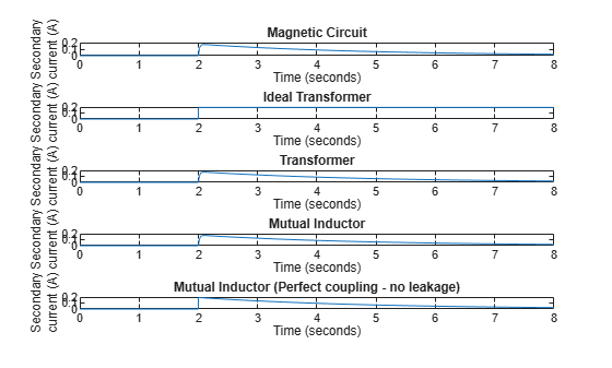
Notice that, as explained above, the Ideal Transformer transmits DC and hence the secondary current does not decay. Furthermore, the change in current is instantaneous due to the main core reluctance dynamics not being modeled. All of the other equivalent circuits do block DC.
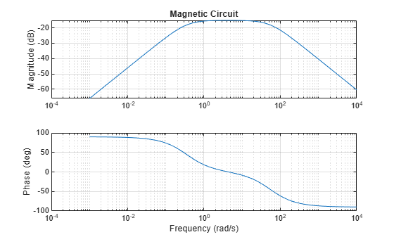
Frequency Response
A better way to view and understand the differences between the different equivalent circuits is to generate a frequency response for each case.
% Linearize the model
sys = linmod("CompareCircuits");

% Bode plot
npts = 100; % Number of points
w = logspace(-3,4,npts); % Vector of frequencies (radians/s)
G = zeros(1,npts); % Frequency response (A/V)
for j=1:5 % Loop over the five equivalent circuits
    for i=1:npts % Determine response at all values in vector w
        G(i) = sys.c(j,:)*(1i*w(i)*eye(size(sys.a))-sys.a)^-1*sys.b(:,j) + sys.d(j,j);
    end
    disp(['Generating Bode plot for the ' titles{j} ' equivalent circuit:'])
    figure
    subplot(2,1,1);
    semilogx(w,20*log10(abs(G)));
    grid on
    ylabel('Magnitude (dB)');
    title(titles{j});
    subplot(2,1,2);
    semilogx(w,180/pi*unwrap(angle(G)));
    ylabel('Phase (deg)');
    xlabel('Frequency (rad/s)');
    grid on
end
Generating Bode plot for the Magnetic Circuit equivalent circuit:
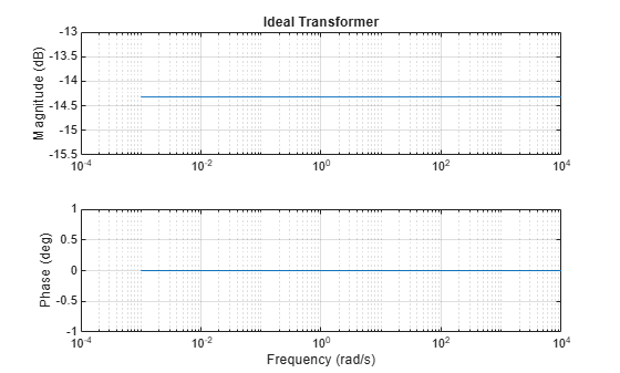
Generating Bode plot for the Ideal Transformer equivalent circuit:
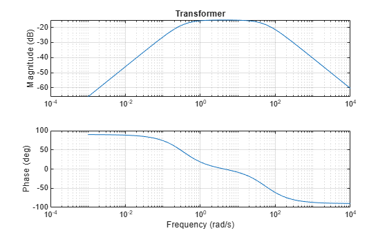
Generating Bode plot for the Transformer equivalent circuit:
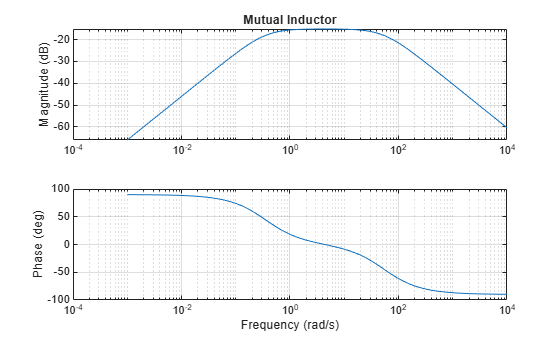
Generating Bode plot for the Mutual Inductor equivalent circuit:
Generating Bode plot for the Mutual Inductor (Perfect coupling - no leakage) equivalent circuit:
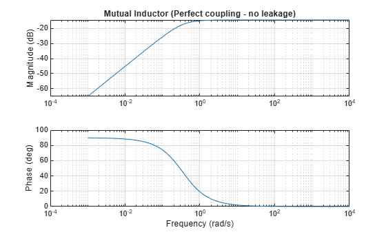
Comparing the frequency plots, you can see that the Magnetic Circuit, Transformer and Mutual Inductor all have identical plots with attenuation at both low and high frequency. However, the Ideal Transformer has no attenuation at low frequency and no attenuation at high frequency, whereas the Mutual Inductor (Perfect coupling - no leakage) attenuates at low frequency, but not at high frequency. These differences are imporant to consider when deciding which block to use when modeling a particular application.