What Is Batch Linearization?
Batch linearization refers to extracting multiple linearizations from a model for various combinations of I/Os, operating points, and parameter values. Batch linearization lets you analyze the time-domain, frequency-domain, and stability characteristics of your Simulink® model, or portions of your model, under varying operating conditions and parameter ranges. You can use the results of batch linearization to design controllers that are robust against parameter variations, or to design gain-scheduled controllers for different operating conditions. You can also use batch linearization results to implement linear parameter varying (LPV) approximations of nonlinear systems using the LPV System block of Control System Toolbox™.
To understand different types of batch linearization, consider the magnetic ball
levitation model, magball. For more information about this model, see
magball Simulink Model.
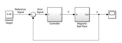
You can batch linearize this model by varying any combination of the following:
I/O sets — Linearize a model using different I/Os to obtain any closed-loop or open-loop transfer function.
For the
magballmodel, some of the transfer functions that you can extract by specifying different I/O sets include:Magnetic ball plant model, controller model
Closed-loop transfer function from the
Reference Signalto the plant output,hOpen-loop transfer function for the controller and magnetic ball plant combined; that is, the transfer function from the
Error Signaltohwith the feedback loop openedOutput disturbance rejection model or sensitivity transfer function, obtained at the outport of
Magnetic Ball Plantblock
Operating points — In nonlinear models, the model dynamics vary depending on the operating conditions. You can linearize a nonlinear model at different operating points to study how model dynamics vary or to design controllers for different operating conditions.
For an example of model dynamics that vary depending on the operating point, consider a simple unforced hanging pendulum with angular position and velocity as states. This model has two equilibrium points, one when the pendulum hangs downward, which is stable, and another when the pendulum points upward, which is unstable. Linearizing close to the stable operating point produces a stable model, whereas linearizing this model close to the unstable operating point produces an unstable model.
For the
magballmodel, which uses the ball height as a state, you can obtain multiple linearizations for varying initial ball heights.Parameters — Parameters configure a Simulink model in several ways. For example, you can use parameters to specify model coefficients or controller sample times. You can also use a discrete parameter, such as the control input to a Multiport Switch block, to control the data path within a model. Therefore, varying a parameter can serve a range of purposes, depending on how the parameter contributes to the model.
For the
magballmodel, you can vary the parameters of the PID Controller block,Controller/PID Controller. The linearizations obtained by varying these parameters show how the controller affects the control-system dynamics. Alternatively, you can vary the magnetic ball plant parameter values to determine the controller robustness to variations in the plant model. You can also vary the parameters of the input block,Desired Height, and study the effects of varying input levels on the model response.If the parameters affect the model operating point, you can batch trim the model using the parameter samples and then batch linearize the model at the resulting operating points.
See Also
Topics
- Choose Batch Linearization Methods
- Batch Linearization Efficiency When You Vary Parameter Values
- Batch Linearize Model for Parameter Value Variations Using Model Linearizer
- Batch Linearize Model for Parameter Variations at Single Operating Point
- Vary Operating Points and Obtain Multiple Transfer Functions Using slLinearizer Interface
- LPV Approximation of Boost Converter Model