Explore Design Reliability Using Parameter Sampling (GUI)
This example shows how to use the Sensitivity Analyzer to explore the behavior of a PI controller for a DC motor. The controller is susceptible to variations caused by component tolerances, and the impact on controller reliability is explored.
You explore the controller reliability by characterizing the components using probability distributions. You use the distributions to generate random samples and perform Monte-Carlo evaluation of the controller design at these sample points. You evaluate the impact of the component tolerances on the controller behavior, and use statistical analysis to determine which components have the most influence on whether the controller meets its requirements. This analysis guides the selection of component tolerances.
This example requires Statistics and Machine Learning Toolbox™.
Implementation of Controller for DC Motor
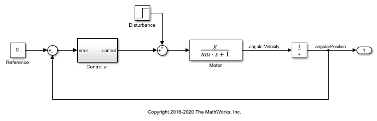
The controller enables the DC motor's angular position to match a desired reference value. The load on the motor is subject to disturbances, and the controller needs to reject these disturbances. The Simulink® model can be used to probe how well the controller rejects a step disturbance at 1 second.
open_system('sdoMotorPosition');
The gains of the PI controller, Kp and Ki, are set using resistors in the circuit below:
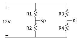
The resistances R1 through R4 are 47 kOhm, 180 kOhm, 10 kOhm and 10 kOhm respectively. These were chosen to set Kp and Ki to values that enable the controller to meet the requirements for disturbance rejection. However, in practice the actual resistor values will differ from the nominal ones, within a tolerance. This raises concern about whether the actual controller will still satisfy the requirements. To explore the effect of different resistance values, use the Sensitivity Analyzer. In the Simulink model from the Apps tab, click Sensitivity Analyzer under Control Systems to open the app.
Design Requirements
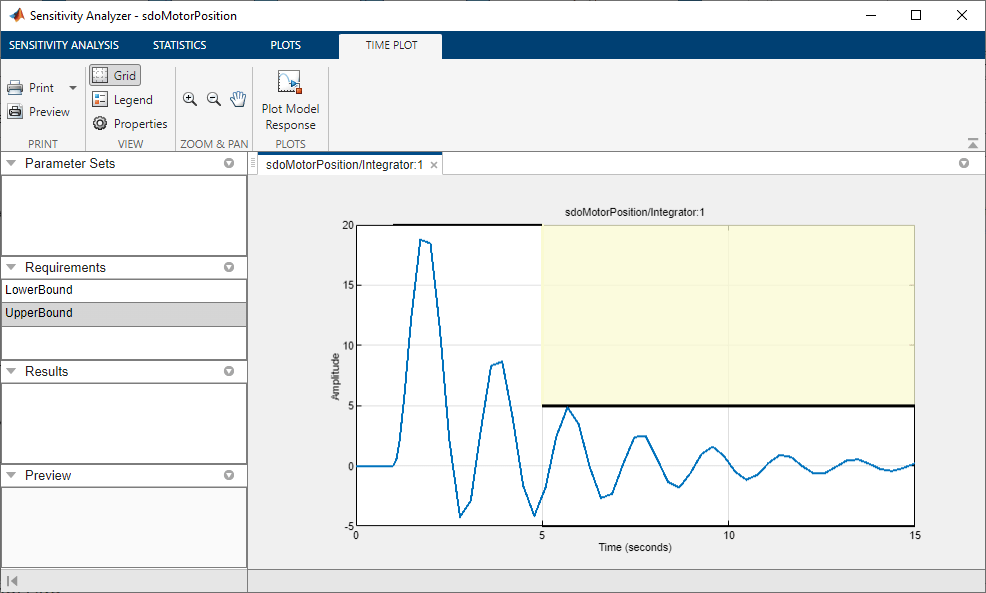
The controller needs to maintain the motor at a reference position in the presence of disturbances. If a step disturbance occurs, the motor needs to deviate no more than 20 degrees, and needs to settle back to within 5 degrees of the reference position by 4 seconds after the disturbance.
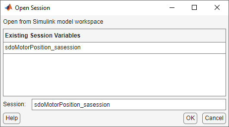
Load previously specified design requirements for disturbance rejection. In the app, click Open Session and select Open from model workspace in the drop-down menu.
You can plot the requirements and verify that they are met when the resistances have the nominal values. In the Requirements area in the data browser, right-click on the LowerBound requirement, and select Plot and Simulate. Do the same for the UpperBound requirement.
Parameter Sampling
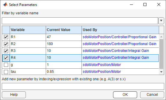
The motor position satisfies the disturbance rejection requirements, when the resistances are at their nominal values. However, in practice the actual resistor values will differ from the nominal ones, and we need to determine whether the controller will still meet the requirements. Click Select Parameters and make a new parameter set. This creates ParamSet in the Parameter Sets area of the app. Specify that R1, R2, R3, and R4 are in the parameter set, and click OK.
Click Generate Values and generate random values. For repeatable results, reset the state of the random number generator in MATLAB®.
rng('default')
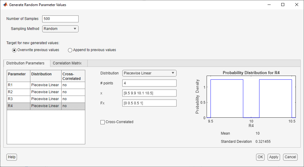
In the Generate Random Parameters dialog box, specify 500 samples to generate.
Specify the probability distribution for each parameter. Standard precision resistors match their nominal component value within a tolerance of 5%. This could be modeled using a uniform probability distribution. However, because resistors that measure within 1% of the nominal value are separated out and sold as higher-priced precision resistors, the 5% resistors can be more accurately modeled by a probability distribution with a well that excludes values within 1% of nominal. This can be modeled using a piecewise linear probability distribution if Statistics and Machine Learning Toolbox™ is available.
Specify the distribution of R1 as piecewise linear with 4 points. Specify the x values as [0.95 0.99 1.01 1.05] times 47 (the nominal value of the resistor). Specify the Fx values as [0 0.5 0.5 1]; these are the values of the cumulative distribution function corresponding to each x value. Similarly, set the distributions of R2, R3 and R4 to piecewise linear with 4 points, the x values as [0.95 0.99 1.01 1.05] times the nominal values (180, 10, and 10, respectively), and the Fx values as [0 0.5 0.5 1].
Click OK to generate parameter values. The generated values are stored in the ParamSet variable in the Parameter Set area of the app. (Note that due to the random number generator, the specific values in the table below may differ from what you get when running the example.)
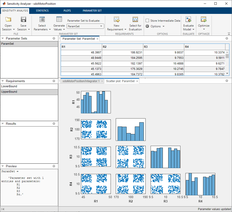
To plot the parameter set click ParamSet in the Parameter Sets area of the app browser. In the Plots tab, select Scatter Plot in the plot gallery. The plot shows the histogram of the generated parameters on the diagonal and pair-wise parameter scatter plots off the diagonal. Each marker on the plot represents one row of the ParamSet table, with each row being simultaneously displayed on all the scatter plots. You can use the View tab to arrange the layout of the table and plot so they are both visible.
Evaluate Requirements with 5% Components
Evaluate the requirements for each row of parameter values in the table to see if the requirements are satisfied. In the Sensitivity Analysis tab, click Select for Evaluation. By default, all requirements are selected to be evaluated. Click Evaluate Model to evaluate the UpperBound and LowerBound requirements for each row of parameter values in ParamSet. Note you can speed up evaluation by using parallel computing if you have the Parallel Computing Toolbox™, or by using fast restart. For more information, see Use Parallel Computing for Sensitivity Analysis and Use Fast Restart Mode During Sensitivity Analysis.
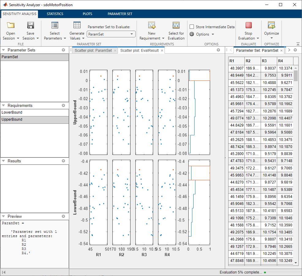
A results scatter plot showing each requirement vs. each parameter is updated during model evaluation. At the end of evaluation a table with the evaluation results is shown. Each row in the evaluation result table contains values for R1, R2, R3, R4 and the resulting requirement values UpperBound and LowerBound. The evaluation results are stored in the EvalResult variable in the Results area of the app. You can use the View tab to arrange the layout of the table and plot so they are both visible.
You can sort the evaluation results table by clicking on the column headers in the table. The LowerBound requirement is still met, as indicated by the fact that all evaluation results for the signal bound requirement are negative. That is not the case for the UpperBound requirement, which has several positive values. By selecting the rows of the table with these positive values, you can also see the corresponding points highlighted in the scatter plot.
Analyze the Evaluation Results
Using 5% tolerance components resulted in violation of the UpperBound requirement. Precision components with 1% tolerance would satisfy the design requirements, but they are more costly, so it is desirable to use only as many as necessary. You can use statistical analysis to identify the components that most influence the design requirements.
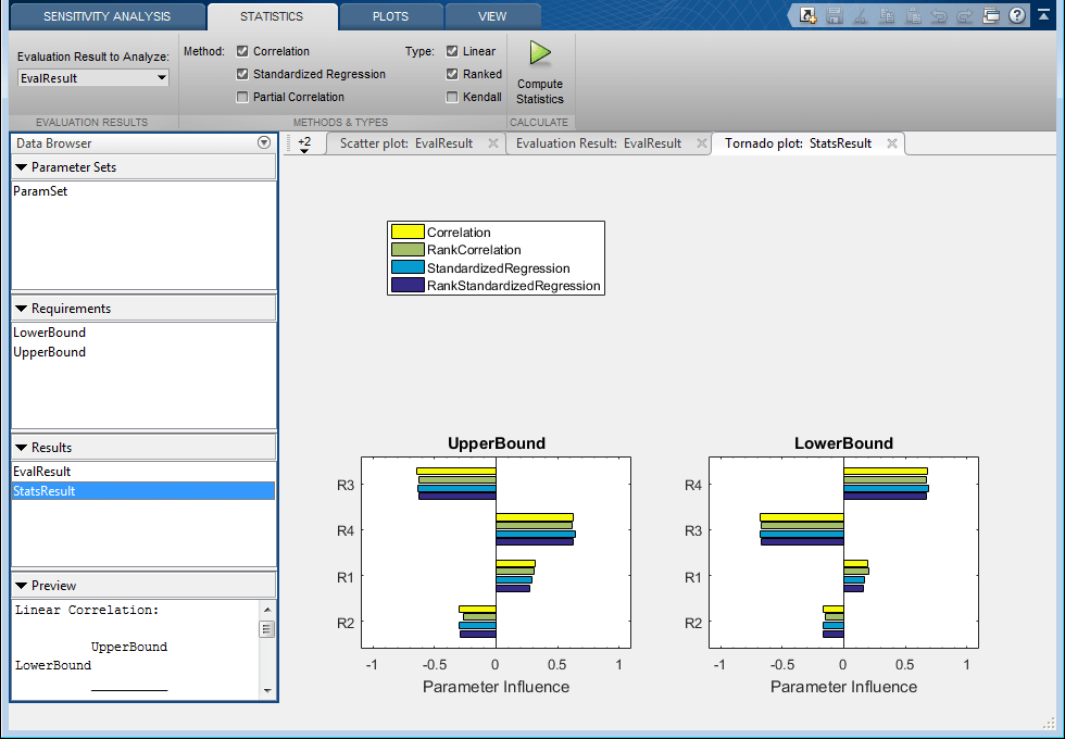
In the Statistics tab, select a variety of analyses to be done, including Correlation and Standardized Regression methods, and Linear and Ranked types of processing. Click Compute Statistics. The analysis result is stored in StatsResult in the Results area of the app, and a tornado plot shows the analysis results. For each requirement, the tornado plot shows the most influential parameters at the top, and the others in decreasing order of the magnitude of their influence on the requirement. For the UpperBound requirement, R3 and R4 have the most influence, so we will try replacing these by higher precision 1% components.
Evaluate Requirements with Mixed Components
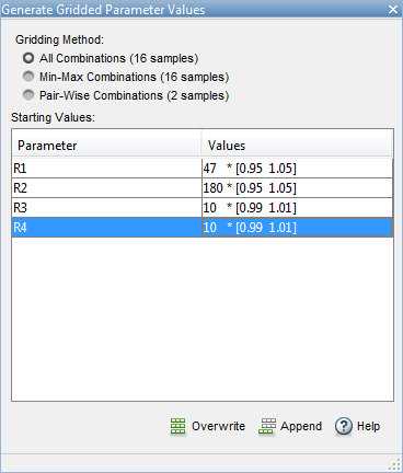
Explore the use of 1% component tolerances only for resistors R3 and R4. In the Sensitivity Analysis tab, click Generate Values and generate gridded values. For R1 and R2, specify that the nominal value is to be perturbed by plus-and-minus 5%. For R3 and R4, specify that the nominal value is to be perturbed by plus-and-minus 1%.
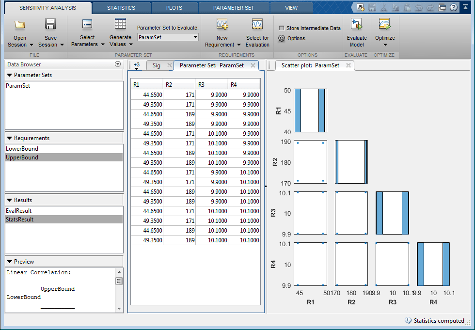
Click Overwrite to generate the new parameter values. To plot the parameter set click ParamSet in the Parameter Sets area of the app browser. In the Plots tab, select Scatter Plot in the plot gallery.
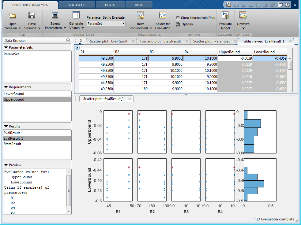
In the Sensitivity Analysis tab, click Evaluate Model. The requirements are evaluated for each row in the table of parameter values, and results are stored in EvalResults_1 shown in the Results area of the app. The evaluation results scatter plot and the evaluation results table show that both requirements are met for all combinations of component values.
The Sensitivity Analyzer was used to explore the effect of standard precision components on the design requirements of a PI controller. With standard precision components, some requirements were found to be violated. Statistical analysis was used to identify which parameters most influence the requirements. The analysis resulted in replacement of only two of the four components with most costly high-precision components.
Close the model.
bdclose('sdoMotorPosition')