Gaussian Process Regression Models
Gaussian process regression (GPR) models are nonparametric kernel-based probabilistic models. You can train a GPR model using the fitrgp function.
Consider the training set , where and , drawn from an unknown distribution. A GPR model addresses the question of predicting the value of a response variable , given the new input vector , and the training data. A linear regression model is of the form
where . The error variance σ2 and the coefficients β are estimated from the data. A GPR model explains the response by introducing latent variables, , from a Gaussian process (GP), and explicit basis functions, h. The covariance function of the latent variables captures the smoothness of the response and basis functions project the inputs into a p-dimensional feature space.
A GP is a set of random variables, such that any finite number of them have a joint Gaussian distribution. If is a GP, then given n observations , the joint distribution of the random variables is Gaussian. A GP is defined by its mean function and covariance function, . That is, if is a Gaussian process, then and
Now consider the following model.
where , that is f(x) are from a zero mean GP with covariance function, . h(x) are a set of basis functions that transform the original feature vector x in Rd into a new feature vector h(x) in Rp. β is a p-by-1 vector of basis function coefficients. This model represents a GPR model. An instance of response y can be modeled as
Hence, a GPR model is a probabilistic model. There is a latent variable f(xi) introduced for each observation , which makes the GPR model nonparametric. In vector form, this model is equivalent to
where
The joint distribution of latent variables in the GPR model is as follows:
close to a linear regression model, where looks as follows:
The covariance function is usually parameterized by a set of kernel parameters or hyperparameters, . Often is written as to explicitly indicate the dependence on .
fitrgp estimates the basis function coefficients, , the noise variance, , and the hyperparameters,, of the kernel function from the data while training the GPR model. You can specify the basis function, the kernel (covariance) function, and the initial values for the parameters.
Because a GPR model is probabilistic, it is possible to compute the prediction
intervals using the trained model (see predict and resubPredict).
You can also compute the regression error using the trained GPR model (see loss and resubLoss).
Compare Prediction Intervals of GPR Models
This example fits GPR models to a noise-free data set and a noisy data set. The example compares the predicted responses and prediction intervals of the two fitted GPR models.
Generate two observation data sets from the function .
rng('default') % For reproducibility
x_observed = linspace(0,10,21)';
y_observed1 = x_observed.*sin(x_observed);
y_observed2 = y_observed1 + 0.5*randn(size(x_observed));
The values in y_observed1 are noise free, and the values in y_observed2 include some random noise.
Fit GPR models to the observed data sets.
gprMdl1 = fitrgp(x_observed,y_observed1);
gprMdl2 = fitrgp(x_observed,y_observed2);
Compute the predicted responses and 95% prediction intervals using the fitted models.
x = linspace(0,10)';
[ypred1,~,yint1] = predict(gprMdl1,x);
[ypred2,~,yint2] = predict(gprMdl2,x);
Resize a figure to display two plots in one figure.
fig = figure;
fig.Position(3) = fig.Position(3)*2;
Create a 1-by-2 tiled chart layout.
tiledlayout(1,2,'TileSpacing','compact')
For each tile, draw a scatter plot of observed data points and a function plot of . Then add a plot of GP predicted responses and a patch of prediction intervals.
nexttile
hold on
scatter(x_observed,y_observed1,'r') % Observed data points
fplot(@(x) x.*sin(x),[0,10],'--r')  % Function plot of x*sin(x)
plot(x,ypred1,'g')                  % GPR predictions
patch([x;flipud(x)],[yint1(:,1);flipud(yint1(:,2))],'k','FaceAlpha',0.1); % Prediction intervals
hold off
title('GPR Fit of Noise-Free Observations')
legend({'Noise-free observations','g(x) = x*sin(x)','GPR predictions','95% prediction intervals'},'Location','best')

nexttile
hold on
scatter(x_observed,y_observed2,'xr') % Observed data points
fplot(@(x) x.*sin(x),[0,10],'--r')   % Function plot of x*sin(x)
plot(x,ypred2,'g')                   % GPR predictions
patch([x;flipud(x)],[yint2(:,1);flipud(yint2(:,2))],'k','FaceAlpha',0.1); % Prediction intervals
hold off
title('GPR Fit of Noisy Observations')
legend({'Noisy observations','g(x) = x*sin(x)','GPR predictions','95% prediction intervals'},'Location','best')
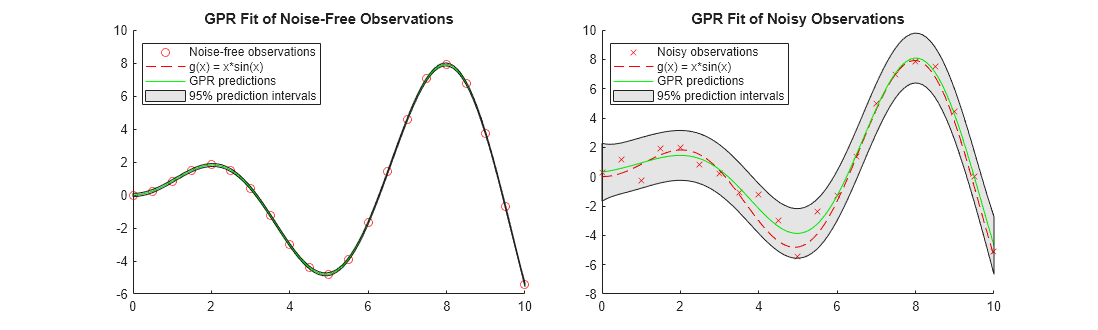
When the observations are noise free, the predicted responses of the GPR fit cross the observations. The standard deviation of the predicted response is almost zero. Therefore, the prediction intervals are very narrow. When observations include noise, the predicted responses do not cross the observations, and the prediction intervals become wide.
References
[1] Rasmussen, C. E. and C. K. I. Williams. Gaussian Processes for Machine Learning. MIT Press. Cambridge, Massachusetts, 2006.
See Also
fitrgp | RegressionGP | predict