divergence
Divergence of symbolic vector field
Description
d = divergence(V,X)V with respect to vector X in
Cartesian coordinates. Vectors V and X
must have the same length.
d = divergence(V)V with respect to a
default vector constructed from the symbolic variables in
V.
Examples
Find the divergence of the vector field with respect to vector .
syms x y z
V = [x 2*y^2 3*z^3];
X = [x y z];
div = divergence(V,X)
div =
Show that the divergence of the curl of the vector field is 0.
divCurl = divergence(curl(V,X),X)
divCurl =
Find the divergence of the gradient of the scalar field . The result is the Laplacian of the scalar field.
syms x y z
f = x^2 + y^2 + z^2;
divGrad = divergence(gradient(f,X),X)
divGrad =
Gauss’s Law in differential form states that the divergence of an electric field is proportional to the electric charge density.
Find the electric charge density for the electric field .
syms x y ep0
E = [x^2 y^2];
rho = divergence(E,[x y])*ep0
rho =
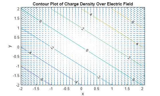
Visualize the electric field and electric charge density for and with ep0 = 1. Create a grid of values of x and y using meshgrid. Find the values of the electric field and charge density by substituting grid values using subs. Simultaneously substitute the grid values xPlot and yPlot into the charge density rho by using cell arrays as inputs to subs.
rho = subs(rho,ep0,1);
v = -2:0.1:2;
[xPlot,yPlot] = meshgrid(v);
Ex = subs(E(1),x,xPlot);
Ey = subs(E(2),y,yPlot);
rhoPlot = double(subs(rho,{x,y},{xPlot,yPlot}));
Plot the electric field using quiver. Overlay the charge density using contour. The contour lines indicate the values of the charge density.
quiver(xPlot,yPlot,Ex,Ey)
hold on
contour(xPlot,yPlot,rhoPlot,"ShowText","on")
title("Contour Plot of Charge Density Over Electric Field")
xlabel("x")
ylabel("y")
Since R2023a
Derive the electromagnetic wave equation in free space without charge and without current sources from Maxwell's equations.
First, create symbolic scalar variables to represent the vacuum permeability and permittivity. Create a symbolic matrix variable to represent the Cartesian coordinates. Create two symbolic matrix functions to represent the electric and magnetic fields as functions of space and time.
syms mu_0 epsilon_0
syms X [3 1] matrix
syms E(X,t) B(X,t) [3 1] matrix keepargs
Next, create four equations to represent Maxwell's equations.
Maxwell1 = divergence(E,X) == 0
Maxwell1(X, t) =
Maxwell2 = curl(E,X) == -diff(B,t)
Maxwell2(X, t) =
Maxwell3 = divergence(B,X) == 0
Maxwell3(X, t) =
Maxwell4 = curl(B,X) == mu_0*epsilon_0*diff(E,t)
Maxwell4(X, t) =
Then, find the wave equation for the electric field. Compute the curl of the second Maxwell equation.
wave_E = curl(Maxwell2,X)
wave_E(X, t) =
Substitute the first Maxwell equation in the electric field wave equation. Use lhs and rhs to obtain the left and right sides of the first Maxwell equation.
wave_E = subs(wave_E,lhs(Maxwell1),rhs(Maxwell1))
wave_E(X, t) =
Compute the time derivative of the fourth Maxwell equation.
dMaxwell4 = diff(Maxwell4,t)
dMaxwell4(X, t) =
Substitute the term that involves the magnetic field in wave_E with the right side of dMaxwell4. Use lhs and rhs to obtain these terms from dMaxwell4.
wave_E = subs(wave_E,lhs(dMaxwell4),rhs(dMaxwell4))
wave_E(X, t) =
Using similar steps, you can also find the wave equation for the magnetic field.
wave_B = curl(Maxwell4,X)
wave_B(X, t) =
wave_B = subs(wave_B,lhs(Maxwell3),rhs(Maxwell3))
wave_B(X, t) =
dMaxwell2 = diff(Maxwell2,t)
dMaxwell2(X, t) =
wave_B = subs(wave_B,lhs(dMaxwell2),rhs(dMaxwell2))
wave_B(X, t) =
Input Arguments
Limitations
The
divergencefunction does not support tensor derivatives. If the inputVis a tensor field or a matrix rather than a vector, then thedivergencefunction returns an error.Symbolic Math Toolbox™ currently does not support the
dotorcrossfunctions for symbolic matrix variables and functions of typesymmatrixandsymfunmatrix. If vector calculus identities involve dot or cross products, then the toolbox displays those identities in terms of other supported functions instead. To see a list of all the functions that support symbolic matrix variables and functions, use the commandsmethods symmatrixandmethods symfunmatrix.