functionalDerivative
Functional derivative (variational derivative)
Description
G = functionalDerivative(f,y)
If y is a vector of symbolic functions,
functionalDerivative returns a vector of functional derivatives with
respect to the functions in y, where all functions in
y must depend on the same independent variables.
Examples
Find the functional derivative of the functional with respect to the function , where the integrand is .
Declare y(x) as a symbolic function and define f as the integrand of . Use f and y as the parameters of functionalDerivative.
syms y(x)
f = y*sin(y);
G = functionalDerivative(f,y)
G(x) =
Find the functional derivative of the functional with respect to the functions and , where the integrand is .
Declare u(x) and v(x) as symbolic functions, and define f as the integrand of .
syms u(x) v(x)
f = u^2*diff(v,x) + v*diff(u,x,x);
Specify a vector of symbolic functions [u v] as the second input argument in functionalDerivative.
G = functionalDerivative(f,[u v])
G(x) =
functionalDerivative returns a vector of symbolic functions containing the functional derivatives of the integrand f with respect to u and v, respectively.
Find the Euler–Lagrange equation of a mass m that is connected to a spring with spring constant k.
Define the kinetic energy T, potential energy V, and Lagrangian L of the system. The Lagrangian is the difference between the kinetic and potential energy.
syms m k x(t)
T = 1/2*m*diff(x,t)^2;
V = 1/2*k*x^2;
L = T - V
L(t) =
In Lagrangian mechanics, the action functional of the system is equal to the integral of the Lagrangian over time, or . The Euler–Lagrange equation describes the motion of the system for which is stationary.
Find the Euler–Lagrange equation by taking the functional derivative of the integrand L and setting it equal to 0.
eqn = functionalDerivative(L,x) == 0
eqn(t) =
eqn is the differential equation that describes mass-spring oscillation.
Solve eqn using dsolve. Assume the mass m and spring constant k are positive. Set the initial conditions for the oscillation amplitude as and the initial velocity of the mass as .
assume(m,'positive')
assume(k,'positive')
Dx(t) = diff(x(t),t);
xSol = dsolve(eqn,[x(0) == 10, Dx(0) == 0])
xSol =
Clear assumptions for further calculations.
assume([k m],'clear')The Brachistochrone problem is to find the quickest path of descent of a particle under gravity without friction. The motion is confined to a vertical plane. The time for a body to move along a curve from point to under gravity is given by
Find the quickest path by minimizing the change in with respect to small variations in the path . The condition for a minimum is .
Compute the functional derivative to obtain the differential equation that describes the Brachistochrone problem. Use simplify to simplify the equation to its expected form.
syms g y(x)
assume(g,'positive')
f = sqrt((1 + diff(y)^2)/(2*g*y));
eqn = functionalDerivative(f,y) == 0;
eqn = simplify(eqn)
eqn(x) =
This equation is the standard differential equation of the Brachistochrone problem. To find the solutions of the differential equation, use dsolve. Specify the 'Implicit' option to true to return implicit solutions, which have the form .
sols = dsolve(eqn,'Implicit',true)sols =
The symbolic solver dsolve returns general solutions in the complex space. Symbolic Math Toolbox™ does not accept the assumption that the symbolic function is real.
Depending on the boundary conditions, there are two real-space solutions to the Brachistochrone problem. One of the two solutions below describes a cycloid curve in real space.
solCycloid1 = sols(3)
solCycloid1 =
solCycloid2 = sols(5)
solCycloid2 =
Another solution in real space is a horizontal straight line, where is a constant.
solStraight = simplify(sols(4))
solStraight =
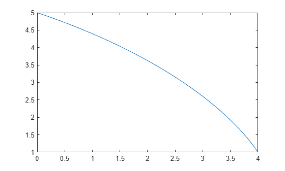
To illustrate the cycloid solution, consider an example with boundary conditions and . In this case, the equation that can satisfy the given boundary conditions is solCycloid1. Substitute the two boundary conditions into solCycloid1.
eq1 = subs(solCycloid1,[x y(x)],[0 5]);
eq2 = subs(solCycloid1,[x y(x)],[4 1]);
The two equations, eq1 and eq2, have two unknown coefficients, and . Use vpasolve to find numerical solutions for the coefficients. Substitute these solutions into solCycloid1.
coeffs = vpasolve([eq1 eq2]);
eqCycloid = subs(solCycloid1,{'C1','C3'},{coeffs.C1,coeffs.C3})
eqCycloid =
The implicit equation eqCycloid describes the cycloid solution of the Brachistochrone problem in terms of and .
You can then use fimplicit to plot eqCycloid. Since fimplicit only accepts implicit symbolic equations that contain symbolic variables and , convert the symbolic function to a symbolic variable . Use mapSymType to convert to . Plot the cycloid solution within the boundary conditions and .
funToVar = @(obj) sym('y');
eqPlot = mapSymType(eqCycloid,'symfun',funToVar);
fimplicit(eqPlot,[0 4 1 5])
For a function that describes a surface in 3-D space, the surface area can be determined by the functional
where and are the partial derivatives of with respect to and .
Find the functional derivative of the integrand f with respect to u.
syms u(x,y)
f = sqrt(1 + diff(u,x)^2 + diff(u,y)^2);
G = functionalDerivative(f,u)
G(x, y) =
The result is the equation G that describes the minimal surface of a 3-D surface defined by u(x,y). The solutions to this equation describe minimal surfaces in 3-D space, such as soap bubbles.
Input Arguments
Output Arguments
More About
Version History
Introduced in R2015a