Replay J1939 Logged Field Data to a Simulation
This example shows how to replay J1939 data from a BLF file acquired from a J1939 system in a real-world application, such as a vehicle running in the field.
The Simulink® model runs a simple horsepower estimator algorithm to trigger a fault that might have occurred in the field*.* The example takes you through a part of the model-based workflow using field data to recreate a fault that was present in the Simulink algorithm before it was deployed onto an ECU, and can be extended to test any algorithm model to debug faults.
J1939 is a higher-layer protocol that uses the Controller Area Network (CAN) bus technology as a physical layer*.* Since CAN is the basis of data transfer in a J1939 system, the tool used in the field by default logs J1939 data as CAN frames. This example performs data replay of the originally logged CAN frames over a CAN bus from MATLAB® and receives in a Simulink model using the J1939 Network Configuration, J1939 Node Configuration, J1939 CAN Transport Layer, and J1939 Receive blocks.
The BLF file used in this example was generated from Vector CANoe using the "System Configuration (J1939)" sample configuration, and modified using MATLAB and Vehicle Network Toolbox™. This example also uses the J1939 DBC file PowerTrain_J1939.dbc, provided with the Vector sample configuration. Vehicle Network Toolbox provides J1939 Simulink blocks for receiving and transmitting parameter groups (PG) via Simulink models over CAN. The example uses MathWorks® virtual CAN channels connected in a loopback configuration.
Read the BLF File Data
Using the blfread function, read the data from channel 1 of the BLF file that was acquired in the field.
canData = blfread("LoggingBLF_J1939Replay.blf",1)canData=15000×8 timetable
Time ID Extended Name Data Length Signals Error Remote
____________ _________ ________ __________ ___________________________________ ______ ____________ _____ ______
0.000568 sec 418316032 true {0×0 char} {[ 76 52 169 232 0 0 0 0]} 8 {0×0 struct} false false
0.001128 sec 418316035 true {0×0 char} {[ 78 52 169 232 0 3 0 0]} 8 {0×0 struct} false false
0.001688 sec 418316043 true {0×0 char} {[ 75 52 169 232 0 9 0 0]} 8 {0×0 struct} false false
0.002244 sec 418316055 true {0×0 char} {[ 77 52 169 232 0 19 0 0]} 8 {0×0 struct} false false
0.002796 sec 418316083 true {0×0 char} {[ 79 52 169 232 0 38 0 0]} 8 {0×0 struct} false false
0.003364 sec 418316262 true {0×0 char} {[ 105 52 169 232 0 131 0 16]} 8 {0×0 struct} false false
0.003932 sec 418316262 true {0×0 char} {[ 105 52 169 232 0 131 0 16]} 8 {0×0 struct} false false
0.25158 sec 201326595 true {0×0 char} {[252 255 255 255 248 255 255 255]} 8 {0×0 struct} false false
0.25216 sec 201326603 true {0×0 char} {[252 255 255 255 248 255 255 255]} 8 {0×0 struct} false false
0.25272 sec 217055747 true {0×0 char} {[ 192 0 0 250 240 240 7 3]} 8 {0×0 struct} false false
0.2533 sec 217056000 true {0×0 char} {[ 1 0 0 0 0 252 0 255]} 8 {0×0 struct} false false
0.25386 sec 217056256 true {0×0 char} {[ 240 0 125 208 7 0 241 0]} 8 {0×0 struct} false false
0.25444 sec 418382091 true {0×0 char} {[ 0 0 0 0 0 1 11 3]} 8 {0×0 struct} false false
0.25501 sec 418383107 true {0×0 char} {[ 125 0 0 125 0 0 0 0]} 8 {0×0 struct} false false
0.2556 sec 418384139 true {0×0 char} {[ 0 0 0 0 0 0 0 0]} 8 {0×0 struct} false false
0.25618 sec 419283979 true {0×0 char} {[ 3 0 0 255 255 255 255 255]} 8 {0×0 struct} false false
⋮
This data contains one PG of interest for this example called EEC1_EMS. The PG contains data coming from the Engine Electronic Controller module. This example manipulates the dataset from the BLF file to deliberately trigger a failure mode for demonstration purposes. The Simulink model recreates this failure using the modified dataset.
Decode and Repackage Parameter Groups to Examine Signal Data
Decode the CAN messages into a J1939 PG timetable.
db = canDatabase("Powertrain_J1939Replay.dbc");
j1939PGTT = j1939ParameterGroupTimetable(canData, db)j1939PGTT=15000×8 timetable
Time Name PGN Priority PDUFormatType SourceAddress DestinationAddress Data Signals
____________ _____________ _____ ________ _____________________ _____________ __________________ ___________________________________ ____________
0.000568 sec ACL 60928 6 Peer-to-Peer (Type 1) 0 255 {[ 76 52 169 232 0 0 0 0]} {1×1 struct}
0.001128 sec ACL 60928 6 Peer-to-Peer (Type 1) 3 255 {[ 78 52 169 232 0 3 0 0]} {1×1 struct}
0.001688 sec ACL 60928 6 Peer-to-Peer (Type 1) 11 255 {[ 75 52 169 232 0 9 0 0]} {1×1 struct}
0.002244 sec ACL 60928 6 Peer-to-Peer (Type 1) 23 255 {[ 77 52 169 232 0 19 0 0]} {1×1 struct}
0.002796 sec ACL 60928 6 Peer-to-Peer (Type 1) 51 255 {[ 79 52 169 232 0 38 0 0]} {1×1 struct}
0.003364 sec ACL 60928 6 Peer-to-Peer (Type 1) 230 255 {[ 105 52 169 232 0 131 0 16]} {1×1 struct}
0.003932 sec ACL 60928 6 Peer-to-Peer (Type 1) 230 255 {[ 105 52 169 232 0 131 0 16]} {1×1 struct}
0.25158 sec TSC1_TECU_EMS 0 3 Peer-to-Peer (Type 1) 3 0 {[252 255 255 255 248 255 255 255]} {1×1 struct}
0.25216 sec TSC1_EBS_EMS 0 3 Peer-to-Peer (Type 1) 11 0 {[252 255 255 255 248 255 255 255]} {1×1 struct}
0.25272 sec ETC1_TECU 61442 3 Broadcast (Type 2) 3 255 {[ 192 0 0 250 240 240 7 3]} {1×1 struct}
0.2533 sec EEC2_EMS 61443 3 Broadcast (Type 2) 0 255 {[ 1 0 0 0 0 252 0 255]} {1×1 struct}
0.25386 sec EEC1_EMS 61444 3 Broadcast (Type 2) 0 255 {[ 240 0 125 208 7 0 241 0]} {1×1 struct}
0.25444 sec EBC1_EBS 61441 6 Broadcast (Type 2) 11 255 {[ 0 0 0 0 0 1 11 3]} {1×1 struct}
0.25501 sec ETC2_TECU 61445 6 Broadcast (Type 2) 3 255 {[ 125 0 0 125 0 0 0 0]} {1×1 struct}
0.2556 sec VDC2_EBS 61449 6 Broadcast (Type 2) 11 255 {[ 0 0 0 0 0 0 0 0]} {1×1 struct}
0.25618 sec EBC5_EBS 64964 6 Broadcast (Type 2) 11 255 {[ 3 0 0 255 255 255 255 255]} {1×1 struct}
⋮
Package the signals from the PG of interest EEC1_EMS into a signal timetable.
sigTable = j1939SignalTimetable(j1939PGTT,ParameterGroups="EEC1_EMS")sigTable=402×7 timetable
Time EngDemandPercentTorque EngStarterMode SrcAddrssOfCtrllngDvcForEngCtrl EngSpeed ActualEngPercentTorque DriversDemandEngPercentTorque EngTorqueMode
___________ ______________________ ______________ _______________________________ ________ ______________________ _____________________________ _____________
0.25386 sec -125 1 0 250 0 -125 0
0.3527 sec -125 1 0 250 0 -125 0
0.4527 sec -125 1 0 250 0 -125 0
0.5527 sec -125 1 0 250 0 -125 0
0.6527 sec -125 1 0 250 0 -125 0
0.7527 sec -125 1 0 250 0 -125 0
0.8527 sec -125 1 0 250 0 -125 0
0.9527 sec -125 1 0 250 0 -125 0
1.0527 sec -125 1 0 250 0 -125 0
1.1527 sec -125 1 0 250 0 -125 0
1.2539 sec -125 1 0 250 0 -125 0
1.3527 sec -125 1 0 250 0 -125 0
1.4527 sec -125 1 0 250 0 -125 0
1.5527 sec -125 1 0 250 0 -125 0
1.6527 sec -125 1 0 250 0 -125 0
1.7527 sec -125 3 0 250 0 -125 0
⋮
Open the Simulink Model
Open the Simulink model that contains your algorithm. The model contained in this example uses a basic J1939 network setup. For more details on this setup and the J1939 blocks, see the example Get Started with J1939 Communication in Simulink.
open demoVNTSL_J1939ReplayExampleans = logical
1
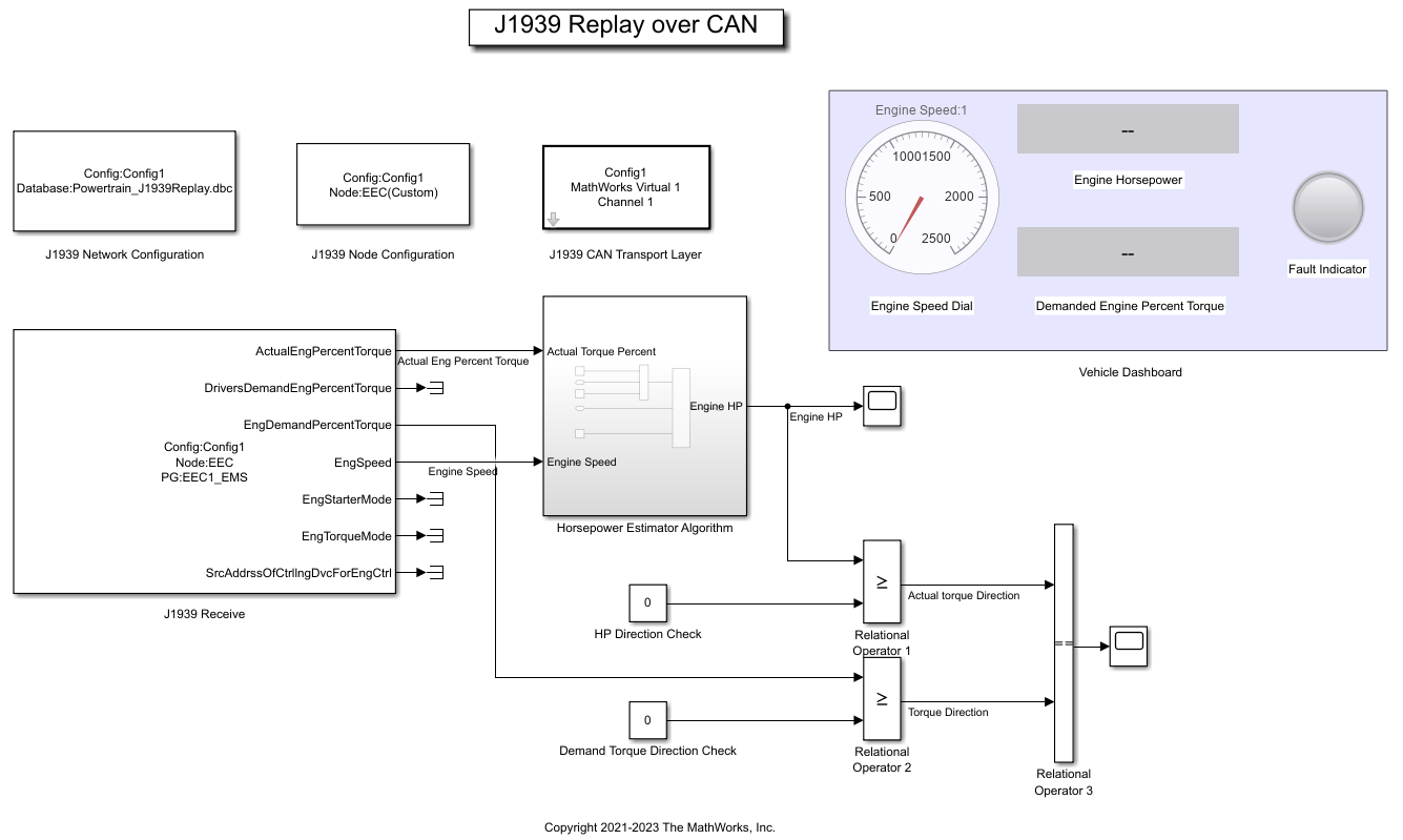
Model Overview
The example model is configured to perform a receive operation for the EEC1_EMS PG over the MathWorks virtual device 1 channel 1.
The J1939 Network Configuration block is configured with the database
Powertrain_J1939.dbc.The J1939 CAN Transport Layer block sets the Device to MathWorks virtual channel 1. The transport layer is configured to transfer J1939 messages over CAN via the specified virtual channel.
The J1939 Receive block receives the messages transmitted over the network. The J1939 Receive is configured to receive the
EEC1_EMSPG and pass on the required inputs (Actual Engine Percentage Torque (%) and Engine Speed (RPM)) to the Horsepower Estimator Algorithm. It is also configured to pass the Engine Demanded Percent Torque (%) to a relational operator block. The rest of the outputs have been terminated for simplicity.
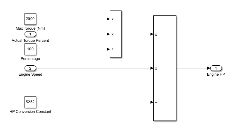
Horsepower Estimator Algorithm
The Horsepower Estimator Algorithm is a simple calculation which takes the actual engine torque percentage and speed values and computes engine horsepower from them.
Relational Operators
There are three relational operator blocks in the model:
Relational Operator 1 compares the value of computed horsepower to zero and outputs a Boolean.
Relational Operator 2 compares the value of engine demanded torque percentage to zero and outputs a Boolean.
Relational Operator 3 compares the value of the outputs from Relational Operators 1 and 2 and outputs a Boolean to trigger the state of the Fault Indicator lamp.
Vehicle Dashboard
The Vehicle Dashboard consists of the speed dial showing the engine RPM, the two gauges showing the computed value of horsepower and the engine percent demanded torque, and the Fault Indicator lamp.
Create the Channel for Replay
Create the CAN channel to replay the messages using the canChannel function.
replayChannel = canChannel("MathWorks","Virtual 1",2);
Set Model Parameters and Start the Simulation
Assign the simulation time and start the simulation.
set_param("demoVNTSL_J1939ReplayExample","StopTime","inf");
set_param("demoVNTSL_J1939ReplayExample","SimulationCommand","start");
Pause until the simulation is fully started.
while strcmp(get_param("demoVNTSL_J1939ReplayExample","SimulationStatus"),"stopped")
end
Start the CAN Channel and Replay the Data
Start the MATLAB CAN channel.
start(replayChannel);
pause(2);
Replay the data acquired from the BLF file. The replay operation runs for approximately 45 seconds.
replay(replayChannel,canData);
Simulation Overview
While this example is running, observe the Simulink model. There will be changes in value in the gauges and the red-green light transition of the Fault Indicator lamp in the Vehicle Dashboard section.
The J1939 Receive block receives the EEC1_EMS PG from MATLAB, decodes the signals of interest, and passes them to the Horsepower Estimator Algorithm. After the horsepower is computed, Relational Operator 1 compares its values to zero to determine the direction. The J1939 Receive block also passes the Engine Demanded Percent Torque to Relational Operator 2. Relational Operator 2 compares its values to zero to determine the direction.
The output is a Boolean 1 if the value is greater than or equal to zero, or 0 if it is less than zero (negative).
Relational Operator 3 takes the outputs of the earlier two relational operators and equates them. If the value for both the blocks is 0 or 1, i.e., positive horsepower and positive torque (1), or negative horsepower and negative torque (0), it provides an output of 1, which in turn triggers the green light of the Fault Indicator lamp. However, if the value for either of the earlier relational operator blocks is opposite to the other one, i.e., positive horsepower (1) and negative torque (0), or negative horsepower (0) and positive torque (1), it provides an output of 0, which in turn triggers the red light of the Fault Indicator lamp. These observations are helpful in determining whether the algorithm is faulty based on the field data, and you can further analyze the algorithm.
Stop the CAN Channel
stop(replayChannel);
Stop the Simulation
set_param("demoVNTSL_J1939ReplayExample","SimulationCommand","stop");