modwtcorr
Multiscale correlation using the maximal overlap discrete wavelet transform
Syntax
Description
wcorr = modwtcorr(w1,w2)w1 and w2. wcorr is
an M-by-1 vector of correlation coefficients, where M is
the number of levels with nonboundary wavelet coefficients. If the
final level has enough nonboundary coefficients, modwtcorr returns
the scaling correlation in the final row of wcorr.
wcorrtable = modwtcorr(___,'table')wcorrtable designate
the type and level of each estimate. For example, D1 designates
that the row corresponds to a wavelet or detail estimate at level
1 and S6 designates that the row corresponds to
the scaling estimate at level 6. The scaling correlation is only computed
for the final level of the MODWT and only when there are nonboundary
scaling coefficients. You can specify the 'table' flag
anywhere after the input transforms w1 and w2.
You must enter the entire character vector 'table'.
If you specify 'table', modwtcorr only
outputs one argument.
[___] = modwtcorr(___,'reflection') reduces the
number of wavelet and scaling coefficients at each scale by half before computing the
correlation. Use this option only when you obtain the MODWT of w1 and
w2 were obtained using the 'reflection' boundary
condition. You must enter the entire character vector 'reflection'. If you
added a wavelet named 'reflection' using the wavelet manager, you must
rename that wavelet prior to using this option.
modwtcorr supports only unbiased estimates of the wavelet correlation.
For these estimates, the algorithm must remove the extra coefficients obtained using the
'reflection' boundary condition. Specifying the
'reflection' option in modwtcorr is identical to first
obtaining the MODWT of w1 and w2 using the default
'periodic' boundary handling and then computing the wavelet correlation
estimates.
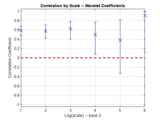
modwtcorr(___) with no output
arguments plots the wavelet correlations by scale with lower and upper
confidence bounds. By default, the coverage probability is 0.95. Scales
with NaNs for the confidence bounds and the scaling correlation are
excluded.
Examples
Find the correlation by scale for monthly DM-USD exchange rate returns from 1970 to 1998. The return data are log transformed. Use the Daubechies wavelet with two vanishing moments ('db2') to obtain the MODWT down to level 6. Then obtain the correlation data.
load DM_USD;
load JY_USD;
wdm = modwt(DM_USD,'db2',6);
wjy = modwt(JY_USD,'db2',6);
wcorr = modwtcorr(wdm,wjy,'db2')
wcorr = 7×1

    0.5854
    0.5748
    0.6264
    0.4948
    0.3787
    0.9072
    0.7976
wcorr contains seven elements. The first six elements are the correlation coefficients for the wavelet (detail) levels one to six. The final element is the correlation for the scaling (lowpass) level six.
Obtain the MODWT of the Southern Oscillation Index and Truk Island daily pressure data sets. Tabulate the correlation between the two data sets by level.
load soi;
load truk;
wsoi = modwt(soi);
wtruk = modwt(truk);
wcorr = modwtcorr(wsoi,wtruk)
wcorr = 10×1

    0.1749
    0.2936
    0.0914
    0.0883
    0.2667
    0.0894
   -0.0415
    0.4825
    0.4394
    0.7433
Show that the number of nonboundary coefficients, in this case, is less than the maximal length of the input. The MODWT is computed down to level thirteen, which is the maximal level for the length of the input. Level thirteen contains thirteen wavelet coefficient vectors and one scaling coefficient vector.
size(wsoi,1)
ans =
14
The multiscale correlations are computed only down to level ten because the levels after than do not contain nonboundary coefficients. For unbiased estimates, you must use nonboundary coefficients only.
numel(wcorr)
ans =
10
Obtain the MODWT of the monthly US-DM and US-JPY exchange return data from 1970 to 1998. The return data are log transformed. Use the Daubechies wavelet with two vanishing moments ('db2') and obtain the MODWT of each series down to level six. Obtain the correlation estimates by scale and the 95% confidence intervals.
load DM_USD
load JY_USD
wdm = modwt(DM_USD,'db2',6);
wjy = modwt(JY_USD,'db2',6);
[wcorr,wcorrci] = modwtcorr(wdm,wjy,'db2');
[wcorr wcorrci]
ans = 7×3

    0.5854    0.4780    0.6756
    0.5748    0.4133    0.7013
    0.6264    0.4016    0.7800
    0.4948    0.0803    0.7634
    0.3787   -0.3295    0.8142
    0.9072    0.1247    0.9939
    0.7976   -0.2857    0.9860
The width of the confidence interval increases as you go down in level.
Specify the coverage probability for the confidence intervals. Obtain the 99% confidence intervals for the US-DM and US-JY exchange returns.
load DM_USD;
load JY_USD;
wdm = modwt(DM_USD,'db2',6);
wjy = modwt(JY_USD,'db2',6);
[wcorr,wcorrci] = modwtcorr(wdm,wjy,'db2',0.99);
[wcorr wcorrci]
ans = 7×3

    0.5854    0.4407    0.7005
    0.5748    0.3557    0.7340
    0.6264    0.3169    0.8153
    0.4948   -0.0646    0.8176
    0.3787   -0.5191    0.8792
    0.9072   -0.3006    0.9975
    0.7976   -0.6227    0.9941
Return p-values for the test of zero correlation by scale. Obtain the MODWT of the DM-USD and JY-USD exchange return data down to level six using the Daubechies wavelet with two vanishing moments ('db2') wavelet. Compute the correlation by scale and return the p-values.
load DM_USD;
load JY_USD;
wdm = modwt(DM_USD,'db2',6);
wjy = modwt(JY_USD,'db2',6);
[wcorr,wcorrci,pval] = modwtcorr(wdm,wjy,'db2');
format longE
pval
pval = 7×2

     2.694174887029554e-17     4.889927419958641e-16
     7.125460513473893e-09     6.466355415977557e-08
     7.012389783536700e-06     4.242495819039703e-05
     2.258540027996925e-02     1.024812537703605e-01
     2.805930327935258e-01     7.275376493146417e-01
     3.348079529469850e-02     1.215352869197555e-01
     1.059217509938030e-01     3.204132967562542e-01
format
The first column contains the p-value and the second column contains the adjusted p-value based on the false discovery rate.
Output results from modwtcorr in tabular form. Obtain the MODWT of the DM-USD and JY-USD exchange returns down to level six using the Daubechies wavelet with two vanishing moments ('db2'). Output the results in a table.
load DM_USD;
load JY_USD;
wdm = modwt(DM_USD,'db2',6);
wjy = modwt(JY_USD,'db2',6);
corrtable = modwtcorr(wdm,wjy,'db2','table')
corrtable=7×6 table
          NJ      Lower        Rho       Upper       Pvalue      AdjustedPvalue
          ___    ________    _______    _______    __________    ______________

    D1    344     0.47797    0.58542    0.67561    2.6942e-17      4.8899e-16
    D2    338     0.41329    0.57483    0.70129    7.1255e-09      6.4664e-08
    D3    326     0.40163    0.62641    0.78001    7.0124e-06      4.2425e-05
    D4    302    0.080255     0.4948    0.76342      0.022585         0.10248
    D5    254    -0.32954    0.37865    0.81417       0.28059         0.72754
    D6    158     0.12469    0.90716    0.99393      0.033481         0.12154
    S6    158    -0.28573    0.79761    0.98601       0.10592         0.32041
Obtain multiscale correlation estimates when using 'reflection' boundary handling. Obtain the MODWT of the Southern Oscillation Index and Truk Islands pressure data sets using 'reflection' boundary handling for both data sets.
load soi
load truk
wsoi = modwt(soi,'fk4',6,'reflection');
wtruk = modwt(truk,'fk4',6,'reflection');
corrtable = modwtcorr(wsoi,wtruk,'fk4',0.95,'reflection','table')
corrtable=7×6 table
           NJ        Lower        Rho       Upper       Pvalue      AdjustedPvalue
          _____    _________    _______    _______    __________    ______________

    D1    12995      0.16942    0.19294    0.21624    1.5466e-55      2.8071e-54
    D2    12989      0.21426    0.24683    0.27885    2.7037e-46      2.4536e-45
    D3    12977     0.057885    0.10623    0.15407     1.789e-05       6.494e-05
    D4    12953     0.048034    0.11645    0.18378    0.00088579       0.0026795
    D5    12905      0.13281     0.2272     0.3175    3.7566e-06      1.7046e-05
    D6    12809    -0.019835     0.1182    0.25181      0.093044         0.24125
    S6    12809      0.26664    0.39003    0.50084    8.8066e-09       5.328e-08
Plot the multiscale correlation of the DM-USD and JY-USD exchange returns down to level six. Use modwtcorr with no output arguments.
load DM_USD;
load JY_USD;
wdm = modwt(DM_USD,'db2',6);
wjy = modwt(JY_USD,'db2',6);
modwtcorr(wdm,wjy,'db2')
Input Arguments
Output Arguments
References
[1] Percival, D. B., and A. T. Walden. Wavelet Methods for Time Series Analysis. Cambridge, UK: Cambridge University Press, 2000.
[2] Whitcher, B., P. Guttorp, and D. B. Percival. “Wavelet analysis of covariance with application to atmospheric time series.” Journal of Geophysical Research, Vol. 105, pp. 14941–14962, 2000.
[3] Benjamini, Y., and Yekutieli, D. “The Control of the False Discovery Rate in Multiple Testing Under Dependency.” Annals of Statistics, Vol. 29, Number 4, pp. 1165–1188, 2001.
Version History
Introduced in R2015b