Signal Multiresolution Analyzer

Decompose signals into time-aligned components

Since R2018b

Description

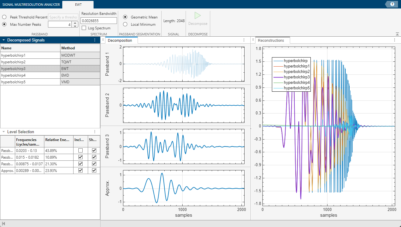
The Signal Multiresolution Analyzer app is an interactive tool for visualizing multilevel wavelet- and data adaptive-based decompositions of real-valued 1-D signals and comparing results. The app supports single- and double-precision data. With the app, you can:

• Access all the real-valued 1-D signals in your MATLAB^® workspace.

• Generate decompositions using fixed-bandwidth and data-adaptive multiresolution analysis (MRA) methods:

  • Fixed-bandwidth: Maximal overlap discrete wavelet transform (MODWT) (default), and tunable Q-factor wavelet transform (TQWT)

  • Data-adaptive: Empirical mode decomposition (EMD), empirical wavelet transform (EWT), and variational mode decomposition (VMD)

• Adjust default parameters, and visualize and compare multiple decompositions.

• Choose decomposition levels to include in the signal reconstruction.

• Obtain frequency ranges of the decomposition levels.

• Determine the relative energy of the signal across levels.

• Export reconstructed signals and decompositions to your workspace.

• Recreate decompositions in your workspace by generating MATLAB scripts.

×

Open the Signal Multiresolution Analyzer App

• MATLAB Toolstrip: On the Apps tab, under Signal Processing and Communications, click the app icon.

• MATLAB command prompt: Enter signalMultiresolutionAnalyzer.

Examples

Visualize Time-Aligned MODWTMRA Decomposition

Load in the Kobe earthquake data. The data are seismograph measurements (vertical acceleration in $\text{nm}/{\text{sec}}^2$) recorded at Tasmania University, Hobart, Australia, on 16 January 1995, beginning at 20:56:51 (GMT) and continuing for 51 minutes at one second intervals.

load kobe

Open Signal Multiresolution Analyzer and click Import. A window appears listing all the workspace variables the app can process.

Select the Kobe data from the dialog box and click Import. By default, a four-level MODWTMRA decomposition of the signal appears in the MODWT tab. The decomposition is obtained using the modwt and modwtmra functions with default settings. The plots in the Decomposition pane are the projections of the wavelet decompositions of the signal at each scale on the original signal subspace. The decomposed signal is named kobe1 in the Decomposed Signals pane. The method MODWT identifies the decomposition. The original signal, kobe, and the reconstruction, kobe1, are plotted in the Reconstructions pane.

By default, plots are with respect to sample index and frequencies are in cycles per sample. To plot with respect to time and display frequencies in hertz, select the Sample Rate radio button on the Signal Multiresolution Analyzer tab. The default sample rate is 1 hertz. The plots and frequencies update to use the sample rate.

The Level Selection pane shows the relative energies of the signal across scales, as well as the frequency bands.

A check box in the Show column controls whether or not that level is displayed in the Decomposition pane. A check box in the Include column controls whether or not to include that level of the wavelet decomposition in the reconstruction. Clicking a plot in the Decomposition pane is another way to include or exclude that level in the signal reconstruction.

To generate a new decomposition, change one of the wavelet parameters in the toolstrip on the MODWT tab and click Decompose.

• Wavelet - Wavelet family

• Number - Wavelet filter number

• Level - Wavelet decomposition level

Changing any parameter in the toolstrip enables the Decompose button.

Compare MODWTMRA and EMD Decompositions

Load the noisy Doppler signal. The signal is a noisy version of the Doppler test signal of Donoho and Johnstone [1].

load noisdopp

Open Signal Multiresolution Analyzer and import the signal into the app. By default, the app creates a four-level MODWTMRA decomposition of the signal in the MODWT tab. In the Decomposed Signals pane, the wavelet decomposition is named noisdopp1. The Reconstructions pane shows the original and reconstructed signals plotted in two different colors.

To add the EMD decomposition, first switch to the Signal Multiresolution Analyzer tab, then click Add ▼ and select EMD.

After a few moments the EMD decomposition noisdopp2 appears in the EMD tab. The decomposition is obtained using the emd function with default settings. The residual is now the thickest plot in the Reconstructions pane. You can change the parameters in the toolstrip and click Decompose to obtain a different EMD decomposition. To learn more about the parameters and the EMD algorithm, see emd.

To more easily see the differences between the two reconstructions, click noisdopp in the plot legend. The text fades, and the plot of the original signal is hidden. You can use the legend to hide any plot in the Reconstructions pane.

Duplicate Decomposition and Generate Script

This example shows how to duplicate a decomposition for modification. The example also shows how to generate a script to recreate the decomposition in your workspace.

Load the Kobe earthquake data into your workspace. The data are seismograph measurements (vertical acceleration in $\text{nm}/{\text{sec}}^2$) recorded at Tasmania University, Hobart, Australia, on 16 January 1995, beginning at 20:56:51 (GMT) and continuing for 51 minutes at one second intervals.

load kobe

Open Signal Multiresolution Analyzer and import the earthquake data into the app. By default, the app creates a four-level MODWTMRA decomposition of the signal called kobe1 using the modwt and modwtmra functions with default settings. To show plots with respect to time and express frequencies in Hz, click the Sample Rate radio button in the Signal Multiresolution Analyzer tab.

Duplicate Decomposition

Create a new six-level decomposition using the order 4 Coiflet. In the Signal Multiresolution Analyzer tab, click Duplicate in the toolstrip. Since kobe1 is the currently selected item in Decomposed Signals, a duplicate of the first decomposition is created. The duplicate is called kobe1Copy. The plots in Reconstructions are updated to include the new decomposition. Except for the color, the duplicate is identical with the first decomposition. You can change the name of the duplicate by right-clicking on the name in Decomposed Signals.

In the MODWT tab, change the settings in the toolstrip to the following values and then click Decompose.

• Wavelet: coif

• Number: 4

• Level: 6

In Level Selection, note which components of the decomposition are included in the reconstruction: the approximation and the level 5 and level 6 details.

Level 4 has approximately 60% of the total energy. Remove levels 5 and 6 from the reconstruction, and include level 4. Show only the approximation and level 4 details in the Decomposition pane. To approximately align the decomposition with the reconstruction, drag the Decomposition pane beneath the Reconstructions pane.

Generate MODWT Script

You have three export options. You can export the reconstruction or the entire decomposition of the selected decomposed signal to your workspace, or you can export a MATLAB™ script to recreate the decomposition in your workspace. To generate a script, in the Signal Multiresolution Analyzer tab click Export > Generate MATLAB Script.

An untitled script opens in your editor with the following executable code. The true-false values in levelForReconstruction correspond to which Include boxes are checked in Level Selection. You can save the script as is, or modify it to apply the same decomposition settings to other signals. Run the code.

% Logical array for selecting reconstruction elements
levelForReconstruction = [false,false,false,true,false,false,true];

% Perform the decomposition using modwt
wt = modwt(kobe,'coif4',6);

% Construct MRA matrix using modwtmra
mra = modwtmra(wt,'coif4');

% Sum down the rows of the selected multiresolution signals
kobe1Copy = sum(mra(levelForReconstruction,:),1);

Plot the original signal and reconstruction. Except for possibly the colors, the plot will match the kobe1Copy reconstruction shown in the app.

t = 0:numel(kobe)-1;
plot(t,kobe)
grid on
hold on
plot(t,kobe1Copy,LineWidth=2)
xlabel("Seconds")
title("Reconstruction")
legend("Original","Reconstruction",Location="northwest")
axis tight
hold off

Generate EMD Script

Add the EMD decomposition of the Kobe data by clicking Add ▼ and selecting EMD in the Signal Multiresolution Analyzer tab. The name of the decomposed signal in the Decomposed Signals pane is kobe3. By default, the reconstruction consists only of the residual. The decomposition is obtained by using the emd function with default settings.

Generate a script that creates the EMD decomposition by clicking Export > Generate MATLAB Script. An untitled script opens in your editor with the following executable code. Run the code.

% Logical array for selecting reconstruction elements
levelForReconstruction = [false,false,false,false,false,true];

% Perform the decomposition using EMD
[imf,residual,info] = emd(kobe, ...
    SiftRelativeTolerance=0.2, ...
    SiftMaxIterations=100, ...
    MaxNumIMF=5, ...
    MaxNumExtrema=1, ...
    MaxEnergyRatio=20, ...
    Interpolation='spline');

% Construct MRA matrix by appending IMFs and residual
mra = [imf residual].';

% Sum down the rows of the selected multiresolution signals
kobe3 = sum(mra(levelForReconstruction,:),1);

Compare the reconstruction kobe3 with the original signal. In this case, the reconstruction only consists of the residual.

plot(t,kobe)
grid on
hold on
plot(t,kobe3,LineWidth=2)
xlabel("Seconds")
title("Reconstruction")
legend("Original","Reconstruction",Location="northwest")
axis tight
hold off

Related Examples

• Visualize and Recreate EWT Decomposition
• Visualize and Recreate TQWT Decomposition
• Visualize and Recreate VMD Decomposition
• Comparing MODWT and MODWTMRA

Parameters

Wavelet — Orthogonal wavelet family

sym (default) | coif | db | fk

Orthogonal wavelet family to use to generate the multiresolution analysis (default), specified as:

• sym — Symlets

• coif — Coiflets

• db — Daubechies wavelets

• fk — Fejér-Korovkin wavelets

The Wavelet parameter is applicable only for generating a multiresolution analysis.

For more information about the wavelets, use the waveinfo function. For example, to learn more about Daubechies wavelets, enter waveinfo('db').

Interpolation — Interpolation method

spline (default) | pchip

Interpolation method to use for envelope construction in empirical mode decomposition, specified as one of the following:

• spline — Cubic spline interpolation

• pchip — Piecewise cubic Hermite interpolating polynomial method

The Interpolation parameter is applicable only for generating an empirical mode decomposition. You can change other options with the app when creating empirical mode decompositions. For more information, see emd.

Programmatic Use

signalMultiresolutionAnalyzer

signalMultiresolutionAnalyzer opens the Signal Multiresolution Analyzer app. Once the app initializes, import a signal for analysis by clicking Import.

signalMultiresolutionAnalyzer(sig)

signalMultiresolutionAnalyzer(sig) opens the Signal Multiresolution Analyzer app and imports, decomposes, and plots the multiresolution analysis of sig using modwtmra and modwt with the sym4 wavelet and default settings.

sig is a variable in the workspace. sig can be:

• A 1-by-N or N-by-1 real-valued vector.

• Single or double precision.

By default, the app plots the decomposition levels as functions of sample index. To plot with respect to time, you can set a sample rate or sample period using the app.

Tips

• To decompose more than one signal simultaneously, run multiple instances of the Signal Multiresolution Analyzer app.

• For the MODWT and TQWT decomposition methods, the script generated by the Signal Multiresolution Analyzer app supports gpuArray (Parallel Computing Toolbox) inputs.

Algorithms

Decomposition Methods

To generate the decompositions, Signal Multiresolution Analyzer uses these functions:

• EMD — emd

• EWT — ewt

• MODWT — modwt and modwtmra

• TQWT — tqwt and tqwtmra

• VMD — vmd

Passband Frequencies

For the fixed-bandwidth methods, MODWT and TQWT, Signal Multiresolution Analyzer reports the theoretical frequency ranges of the decomposition levels. For the data-adaptive methods, EMD, EWT, and VMD, the app reports the measured bandwidth.

References

[1] Percival, Donald B., and Andrew T. Walden. Wavelet Methods for Time Series Analysis. Cambridge Series in Statistical and Probabilistic Mathematics. Cambridge ; New York: Cambridge University Press, 2000.

Version History

Introduced in R2018b