Wavelet Signal Analyzer

Analyze and compress signals using wavelets

Since R2023a

Description

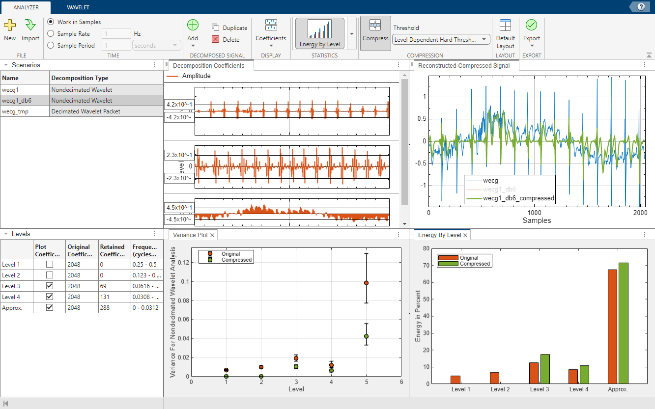
The Wavelet Signal Analyzer app enables visualization, analysis, and compression of 1-D signals using the nondecimated discrete wavelet transform. The app plots the decomposition of the signal and its corresponding reconstruction. The app also shows statistics of the decomposition, including the approximate frequency band of each component. With the Wavelet Signal Analyzer app, you can:

Access all single-channel, real- and complex-valued 1-D signals in the MATLAB^® workspace
Compare reconstructions from different analyses by varying the wavelet or the decomposition level
Visualize the time-aligned coefficients
Extend the signal periodically or by reflection before computing the wavelet transform
Apply a threshold to the wavelet coefficients to compress the signal
Plot the energy for all decomposition levels and display histograms of the original and compressed coefficients at a specific level
Export decomposition coefficients, compressed coefficients, and compressed signals to the MATLAB workspace
Generate MATLAB scripts to reproduce results in your workspace

The Wavelet Signal Analyzer app supports single- and double-precision data.

Open the Wavelet Signal Analyzer App

MATLAB Toolstrip: On the Apps tab, under Signal Processing and Communications, click the app icon.
MATLAB command prompt: Enter waveletSignalAnalyzer.

Examples

expand all

Visualize Wavelet Decomposition Using Wavelet Signal Analyzer

Open Live Script

This example shows how to use the Wavelet Signal Analyzer app to visualize the wavelet decomposition of a 1-D signal using the nondecimated discrete wavelet transform.

Import Data

Load an electroencephalogram (ECG) signal.

load wecg

Visualize Wavelet Decomposition

Open Wavelet Signal Analyzer. On the Analyzer tab, click Import. A window appears with a list of all the workspace variables the app can process. Select wecg and click Import. A four-level nondecimated wavelet decomposition of the signal appears. The decomposed signal is named wecg1 in the Scenarios pane. The decomposition type Nondecimated Wavelet identifies the decomposition. The original signal, wecg, and the reconstruction, wecg1, are plotted in the Reconstructed-Compressed Signal pane. By default, the plots are identical. To hide the plot of the original signal, click wecg in the plot legend. The text fades and the plot of the original signal disappears. You can use the legend to hide any plot in the Reconstructed-Compressed Signal pane.

The plots in the Decomposition Coefficients pane are the amplitudes of the coefficients of the wavelet decomposition of the signal at each scale. To compress the signal, you can threshold the coefficients in the plots. For more information, see Compress Signal and Generate Script. To plot the magnitudes or the sorted magnitudes of the coefficients, choose the desired option from the Coefficients ▼ menu on the Analyzer tab.

By default, plots are with respect to sample index and frequencies are in cycles per sample. To specify a sample rate, select the Sample Rate radio button on the Analyzer tab. The default sample rate is 1 hertz. To instead specify a sample period, select the Sample Period radio button. The default sample period is 1 second. Plots update automatically to reflect how you specify time.

For each scale, the Levels pane shows: the number of coefficients, the number of nonzero coefficients, and the approximate frequency band. The frequency units depend on how you specify time. A check box in the Plot Coefficients column controls whether to plot the coefficients in the Decomposition Coefficients pane.

Plot Histogram

To plot a histogram of the coefficients, click Histogram on the Analyzer tab. The Histogram tab appears, and a histogram of the level 1 coefficients is shown in the Histogram pane. To choose a different level, use the Histogram Level ▼ menu in the toolstrip. For example, to plot the histogram of the level 3 coefficients, select Level 3 from the menu. In the toolstrip, you can also specify a different histogram bin width and normalization scheme.

Plot Energy by Level

The nondecimated discrete wavelet transform partitions the energy of the signal across all levels. To plot the energy percentage of all levels, in the Analyzer tab, select Energy by Level from the Histogram ▼ menu.

Modify Wavelet Transform Parameters

To access the parameters used to generate the decomposition, click the Wavelet tab. The parameters correspond to input arguments of the modwt function. Parameter settings are the default values. To generate a new decomposition, change one or more of the parameters and click Analyze. All plots, such as the histogram, update.

Wavelet — Wavelet family
Number — Wavelet filter number
Level — Decomposition level
Boundary — Specify boundary handling condition
Time Align — Circularly shift the wavelet coefficients at all levels (scales) and the scaling coefficients to correct for the delay of the scaling and wavelet filters

Note: Checking the Time Align checkbox is strictly only for visualization purposes. The plotted reconstruction is always from the original coefficients, and not the time-aligned coefficients. Similarly, compressed signals are based on the thresholded original coefficients. Only original or thresholded coefficients are exported.

Changing any parameter in the toolstrip enables the Analyze button. For more information about the parameters, see modwt.

Export Decomposition

To export the decomposition of the selected scenario to your MATLAB™ workspace, on the Analyzer tab, choose To Workspace under Decomposition Coefficients in the Export ▼ menu. The variable scenarioNameDecomposition is created. If a variable of the same name already exists in the workspace, the app gives you the option to overwrite it. For example, exporting the decomposition for the scenario wecg1 creates the workspace variable wecg1Decomposition.

Compress Signal and Generate Script

Open Live Script

This example shows how to compress a signal and generate a script to recreate the compressed signal in the workspace.

Import Data

Load the electrical consumption signal.

load nelec

Open Wavelet Signal Analyzer and import the signal into the app. By default, a four-level nondecimated wavelet decomposition of the signal appears. The table in the Levels pane indicates there are 2000 original and retained coefficients at all levels.

Inspect the histograms of the coefficients at all levels. The approximation coefficients are in the interval [100, 500]. Observe that at levels 1 through 4, most wavelet coefficients are in the interval [–10, 10].

Apply Threshold

On the Analyzer tab, click Compress. The app applies a default threshold thr to the coefficients. All coefficients that lie in the interval [–thr, thr] are set to 0.

The Levels pane reports the number of coefficients retained at each level after thresholding.
The Histogram pane updates to include the retained coefficients.
The Reconstructed-Compressed Signal pane now includes a plot of the compressed signal, nelec1_compressed. Click nelec and nelec1 in the plot legend to show only the compressed signal.

To apply a different threshold thr, click the Decomposition Coefficients pane. In any level coefficients plot, you can either drag the horizontal cursor to the desired threshold or enter the threshold in the cursor text field. The same threshold is applied to coefficients at all levels. Instead of thresholding plots of the coefficient amplitudes, you can choose a different plot style. In the Coefficients ▼ menu, select Sorted Magnitude and Thresholded Coefficients. Specify a threshold of 250. The plot of the compressed signal updates, as do the values in the Level pane, and histogram.

If you want to compress a signal using two different thresholds and compare the results, on the Analyzer tab, click Duplicate. A second scenario, nelec1Copy, appears in the Scenarios pane. Select the new scenario and apply the second threshold. You can then alternate selected scenarios to compare the compressed signal plots.

Generate Script

You have a number of export options available. You can export the original coefficients or generate a script to recreate the decomposition in your workspace. Because compression is enabled, you can also export the compressed signal or thresholded coefficients, as well as generate a script to recreate the compressed signal in your workspace. To recreate the compressed signal in your workspace, in the Export ▼ menu, choose Generate MATLAB™ Script under Compressed Signal.

An untitled script opens in your editor with the following executable code. You can save the script as is or modify it to apply the same compression to other signals. Run the code.

Note: The generated script always uses the original coefficients. Checking the Time Align checkbox in the Wavelet tab is strictly only for visualization purposes. The state of the checkbox has no impact on the generated script.

% Perform the decomposition using modwt
wt = modwt(nelec,'sym4',4);

numberOfLevelsPlusOne = size(wt,1);

% Compute the energy by level for the decomposition
energyByLevel = 100*sum((wt.^2),2)/sum(wt.^2,'all');

% Thresholds for compressing the imported signal
compressionThresholds = repmat(250, 1, numberOfLevelsPlusOne);

% Duplicate coefficients for thresholding
wc = wt;

for idx = 1:numel(compressionThresholds)
    thr = compressionThresholds(idx);
    w = wc(idx,:);
    w(abs(w) <= abs(thr)) = 0;
    wc(idx,:) = w;
end

% Energy by level for the compressed signal
energyByLevelForCompressed = 100*sum((wc.^2),2)/sum(wc.^2,'all');

% Compute the compressed signal
nelec1_compressed = imodwt(wc,'sym4');

Plot the original signal, nelec, and the compressed signal, nelec1_compressed. Except for possibly the colors, the plots match those shown in the app.

plot(nelec)
hold on
plot(nelec1_compressed,LineWidth=2)
hold off
axis tight
title("Original and Compressed Signals")
legend("Original","Compressed")

Figure contains an axes object. The axes object with title Original and Compressed Signals contains 2 objects of type line. These objects represent Original, Compressed.

Compare the energies by level of the original and thresholded coefficients. Because all the wavelet (detail) coefficients have been set to 0, all of the energy in the thresholded coefficients is contained in the approximation level.

[energyByLevel energyByLevelForCompressed]

ans = 5×2

    0.0152         0
    0.0124         0
    0.0125         0
    0.0260         0
   99.9338  100.0000

Visualize Wavelet Decomposition of Complex-Valued Signal

Open Live Script

Load the NPG2006 dataset. Extract the complex-valued signal from the npg2006 structure array.

load npg2006
npgdata = npg2006.cx;

Open Wavelet Signal Analyzer and import the signal into the app. A four-level nondecimated wavelet decomposition of the signal appears. By default, the app plots the real and imaginary parts of the decomposition and reconstruction.

Show the histogram of the level 3 coefficients. Because the decomposition is complex valued, the app shows separate histograms of the real and imaginary parts of the coefficients.

Show the energy by level. Most of the energy is concentrated in the approximation coefficients.

Specify a threshold thr and compress the signal. Coefficients whose magnitudes are in the interval [–thr, thr] are set to 0. You can specify a threshold in a coefficients plot of any style: amplitude, magnitude, or sorted magnitude. For convenience, set the threshold in the plot of the sorted magnitudes of the coefficients. Show the thresholded coefficients. Show only the real part of the original and compressed signals.

Programmatic Use

expand all